Ocean Optics NanoCalc User Manual

Page 39

Ocean Optics Germany GmbH Thin Film Metrology

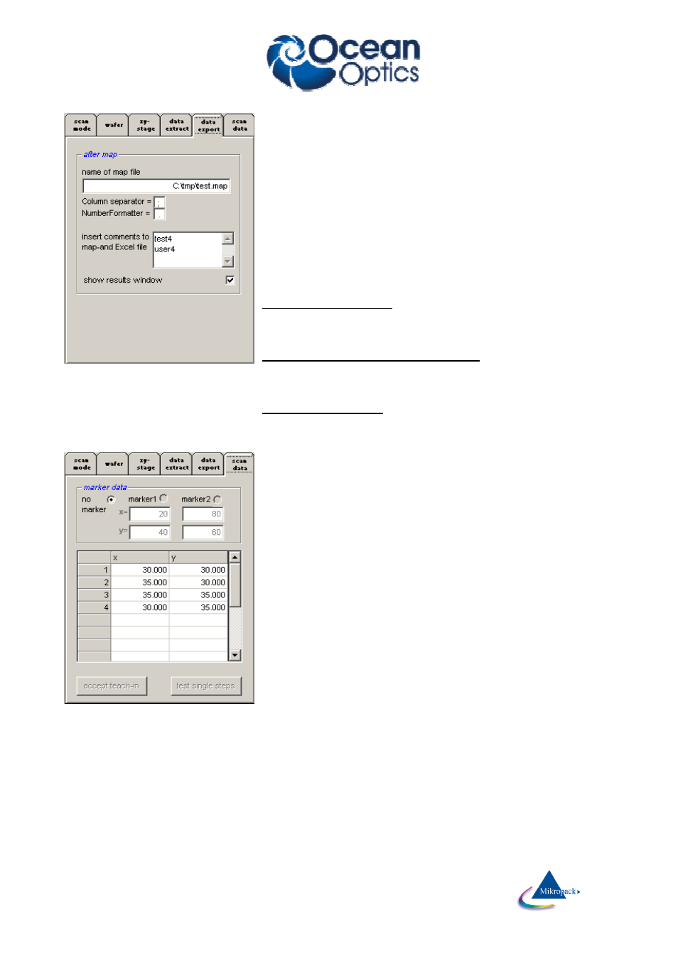
data export:
You may choose the following options during a mapping experiment:

1. plot the simulated curve
2. plot thickness value

It is more informative to see the analyzed curve and the calculated value of
thickness during the simulation, but this is time-consuming. If the mapping
takes a longer time it is recommended to switch off these 2 features.

You may choose the following options after a mapping experiment:

1. write data as map-file
2. insert comments in map or Excel-files
3. show results window

1. Write data as map-file

All thickness and fitness data together with some coordinate information
are written to a ASCII-file in directory “NanoCalc\data\map_files”.
examples can be found in the directory “NanoCalc\data\map_Files”

2. insert comments in map or Excel-files

You may enter text like “sample #1, “Paul McCartney” or “myfirsttest”.
This text will be a header for your map-files and also for all exported
Excel_files

3. show result window

If you accept this option a results window with possibility for Excel export
will open after the mapping process.

Scan data:
This feature is used in microscope arrangement (e.g. for measuring struc-
tured wafers) if you want to hit the xy-positions with higher accuracy.
Usually the wafer or sample will be positioned on the chuck with some
mechanical adjustments (like pins on 2 sides of the wafer and adjustment to
the wafer flat). This will result in a medium accuracy, but not comparable to
fine positioning like in semiconductor photolithography.

How to get a higher accuracy:
1. click on “marker 1”:
The stage will move to this position. If you now look through the

microscope you will see a slight deviation between the illuminated spot
and the real marker on your wafer.

2. Correct this deviation by moving the stage (use the keyboard arrows:

clicking or pressing once = 10 micrometer, SHIFT + clicking or pressing
once = 1 millimeter). The red circle on the screen will move slightly off the
marker.

3. Repeat step 1 and 2 for marker 2
4. Now the software knows both deviations and is able to calculate what to

do: shifting the origin and rotating the scan pattern a little bit. Press the
button: “accept teach-in”

5. Control the values of rotation angle and xy-origin
6. Start mapping as usual