Pitney Bowes MapInfo Vertical Mapper - Manual (Page 59)

Chapter 4: Creating Grids Using Spatial Models
User Guide
57
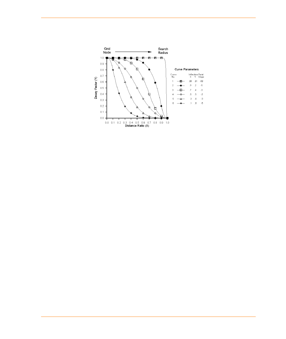
distance decay curves, as shown in the next figure, the slope is zero where x = 0 and gradually
decreases, becoming more negative, until the inflection point is reached. At this point, the slope
gradually increases, becoming more positive and returning to zero again as x approaches one.
Shown here are six search radius distance decay curves supported by the Location
Profiler. Values along the x-axis represent a ratio obtained by dividing the distance
between the grid point and data point by the search radius. Curve 3 represents the
most typical search radius decay function that can be applied to the widest variety of
modeling parameters.
A similar decay function can be applied to the exclusion zone of the grid cell but using a curve with a
positive slope. In this case, the slope is zero where x=0 and gradually increases, becoming more
positive, until the inflection point is reached and then gradually decreases and returns to zero as x
approaches one.
Various methods can be used to obtain the distributions shown in the following figures. Most
techniques require that you specify the location (x- and y- coordinates) of the inflection point and the
slope at this inflection point. Given an appropriate distance decay curve, a decay factor can
therefore be determined for any distance value measured between the grid cell and a weighted point
location. When x = 0 (at the grid cell assuming no exclusion radius setting), then y = 1 (no distance
decay factor), and the slope is 0. When x=1 (at the outer edge of the search radius), then y = 0 (100
percent decay), and again the slope is 0.