HP 50g Graphing Calculator - Manual (Page 536)

Page 16-59
@@OK@@ @INIT+—.75 @@OK@@ ™™@SOLVE (wait) @EDIT
(Changes initial value of t to 0.5, and final value of t to 0.75, solve for v(0.75)
= 2.066…)
@@OK@@ @INIT+—1 @@OK@@ ™ ™ @SOLVE (wait) @EDIT
(Changes initial value of t to 0.75, and final value of t to 1, solve for v(1) =
1.562…)
Repeat for t = 1.25, 1.50, 1.75, 2.00. Press
@@OK@@ after viewing the last result in
@EDIT. To return to normal calculator display, press $ or L@@OK@@. The
different solutions will be shown in the stack, with the latest result in level 1.
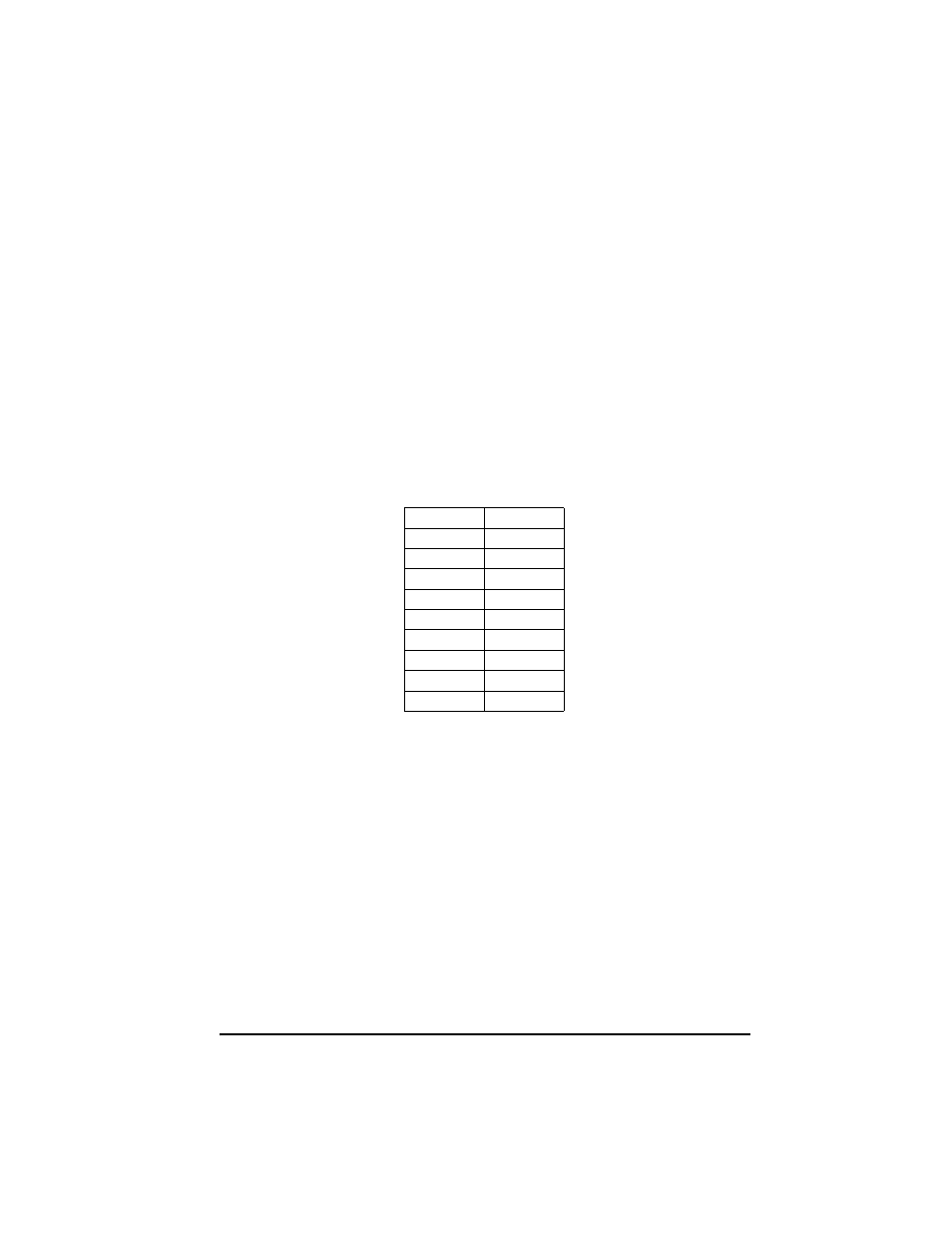
The final results look as follows (rounded to the third decimal):
Graphical solution of first-order ODE
When we can not obtain a closed-form solution for the integral, we can always
plot the integral by selecting Diff Eq in the TYPE field of the PLOT
environment as follows: suppose that we want to plot the position x(t) for a
velocity function v(t) = exp(-t
2
), with x = 0 at t = 0. We know there is no
closed-form expression for the integral, however, we know that the definition of
v(t) is dx/dt = exp(-t
2
).
The calculator allows for the plotting of the solution of differential equations of
the form Y'(T) = F(T,Y). For our case, we let Y = x and T = t, therefore, F(T,Y) =
f(t, x) = exp(-t
2
). Let's plot the solution, x(t), for t = 0 to 5, by using the following
keystroke sequence:
t v
0.00 4.000
0.25 3.285
0.50 2.640
0.75 2.066
1.00 1.562
1.25 1.129
1.50 0.766
1.75 0.473
2.00 0.250