HP 48gII - Manual (Page 544)

Page 16-66
Repeat for t = 1.25, 1.50, 1.75, 2.00. Press @@OK@@ after viewing the last result
in @EDIT. To return to normal calculator display, press $ or L@@OK@@. The
different solutions will be shown in the stack, with the latest result in level 1.
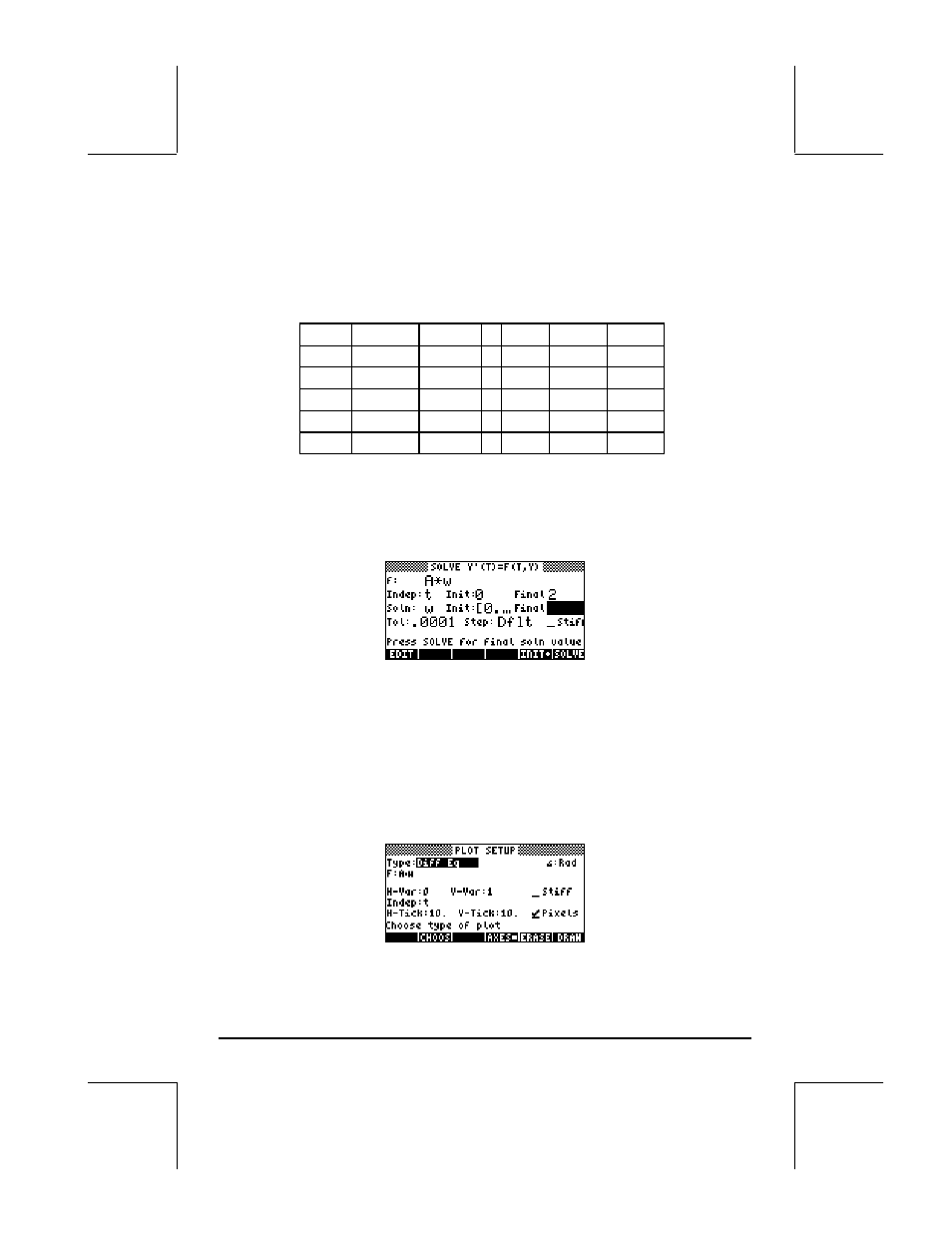
The final results look as follows:
t x x' t x x'
0.00 0.000 6.000 1.25 -0.354 1.281
0.25 0.968 1.368 1.50 0.141 1.362
0.50 0.748 -2.616 1.75 0.227 0.268
0.75 -0.015 -2.859 2.00 0.167 -0.627
1.00 -0.469 -0.607
Graphical solution for a second-order ODE
Start by activating the differential equation numerical solver, ‚ Ï
˜ @@@OK@@@ . The SOLVE screen should look like this:
Notice that the initial condition for the solution (Soln: w Init:[0., …) includes
the vector [0, 6]. Press
L @@OK@@.
Next, press
„ô (simultaneously, if in RPN mode) to enter the PLOT
environment. Highlight the field in front of TYPE , using the —˜keys.
Then, press @CHOOS, and highlight Diff Eq, using the —˜keys. Press
@@OK@@. Modify the rest of the PLOT SETUP screen to look like this: