HP 48gII - Manual (Page 538)

Page 16-60
0 HERMITE, result: 1, i.e., H
0
* = 1.
1 HERMITE, result: ’2*X’, i.e., H
1
* = 2x.
2 HERMITE, result: ’4*X^2-2’, i.e., H
2
* = 4x 2 -2.
3 HERMITE, result: ’8*X^3-12*X’, i.e., H
3
* = 8x 3 -12x.
Numerical and graphical solutions to ODEs
Differential equations that cannot be solved analytically can be solved
numerically or graphically as illustrated below.
Numerical solution of first-order ODE
Through the use of the numerical solver ( ‚Ï), you can access an input
form that lets you solve first-order, linear ordinary differential equations. The
use of this feature is presented using the following example. The method used
in the solution is a fourth-order Runge-Kutta algorithm preprogrammed in the
calculator.
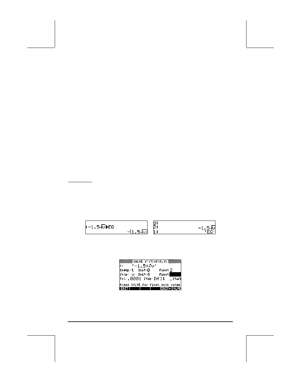
Example 1 -- Suppose we want to solve the differential equation, dv/dt = -1.5
v
1/2 , with v = 4 at t = 0. We are asked to find v for t = 2.
First, create the expression defining the derivative and store it into variable
EQ. The figure to the left shows the ALG mode command, while the right-
hand side figure shows the RPN stack before pressing
K.
Then, enter the NUMERICAL SOLVER environment and select the differential
equation solver:
‚Ϙ @@@OK@@@ . Enter the following parameters: