Measurement Computing eZ-TOMAS version 7.1.x - Manual (Page 61)

eZ-TOMAS & eZ-TOMAS Remote 928192 Toolbar Buttons 6-3
3
rd
Toolbar (continued)
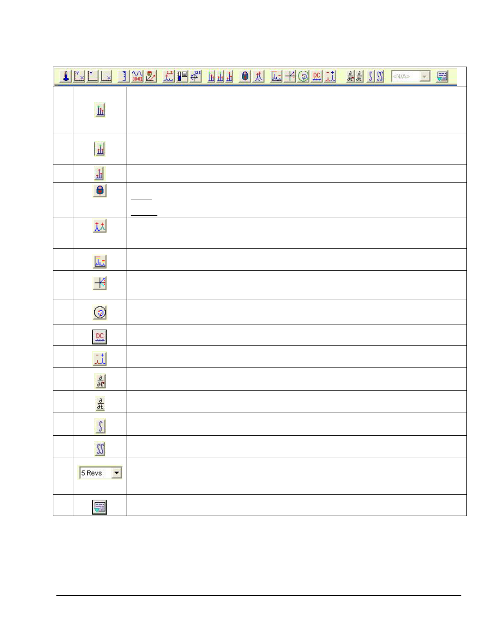
11 Harmonic Cursors – Can only be used when 1 trace is displayed. Results in several cursors positioned to the right of
the primary cursor and at intervals that are at twice the x-axis value of the primary cursor. For example: When the
primary cursor is at 100 Hz, the first harmonic cursor will be at 200 Hz, the second at 400 Hz, the third at 600 Hz, etc.
Moving the primary cursor to 400 Hz would result in the first harmonic cursor residing at 800 Hz, the second at 1200
Hz, etc. If Display Gauge Values is selected, the applicable values will be shown for all cursors. Harmonic cursors
can only be moved by moving the primary cursor.
12 Side Band Cursors – Can only be used when 1 trace is displayed. Results in several cursors spaced at even
intervals on both sides of the primary cursor. Unlike the harmonic cursors, the sideband cursors can be moved by
the user. Once adjusted, they remain in position at until the next adjustment. If Display Gauge Values is selected,
the applicable values will be shown for all cursors.
13 Peak Cursors – Can only be used when 1 trace is displayed. The cursors will automatically position at the highest
peaks on the trace.
14 Multiple Trace Cursor
Locked - When locked, cursors for like plots are moved simultaneously. As you move cursors in one spectrum, the
cursors in the other spectrum plots move to the same X position.
Unlocked - When unlocked, you can only move the cursors in the plot that has focus.
15 Cursor Update - Fixed X axis / Peak Search – When this button has a gray background, the x-axis is fixed and the
cursor will not move when a new spectrum is plotted. When the button has a green background “Peak Search” is in
effect and the cursor will automatically move to the highest point on the plot. The button is typically used for
Spectrum plots, either Real Time or Historical Data.
16 Overlay Limits – For Spectrum, Stripchart, and Polar plot windows. Superimposes the limit values onto the
displayed data.
17 Runout Compensation – displays a graph of the RunOut compensated values for Bode and Polar plots. RunOut
compensation is a vector math operation in which the referenced first-order amplitude and phase vector is subtracted
from the displayed first order vector. For Time Waveform and Orbit plots this shows time waveform compensation.
18 Overlay Bearing Clearance Circle – For Orbit and Shaft Centerline this button is used to superimpose the bearing
clearance circle over the plot display.
19 Apply DC Coupling – For Bode, Stripchart, and Time Waveform this button is used to apply DC Coupling.
Commonly used with Displacement Probes.
-/+ Spectrum Full – Sets the x-axis to have both negative and positive on the scale.
20 Double Differential – Changes the display by a double differential, for example, from Displacement to
Accelerometer.
21 Single Differential – Changes the display by a single differential, for example, from Displacement to Velocity, or
Velocity to Accelerometer.
22 Single Integration – Changes the display by a single integration, for example, from Velocity to Displacement, or
from Accelerometer to Velocity.
23 Double Integration – Changes the display by a double integration, for example, from Accelerometer to
Displacement.
24 Shaft Revolution Filter – Used with Time and Orbit plots. This filter selection is used to limit the amount of data
displayed. The limitation is set by selecting “n,” where “n” is equal to the number of shaft revolutions. The Shaft
Revolution Filter is used to make the plot display cleaner by reducing clutter from excess data. Selection options are:
N/A, 1 rev, 2 revs, 5 revs, and 10 revs.
25 Show User Notes – Displays the User Notes from the Project Information window. The notes are displayed in a
free-moving, re-sizeable box. You can enter text in this field.