Casio 330 - Manual (Page 212)

20090601
2-8-52
Using the Action Menu
Menu Item: [Action][Inv. Distribution][invChiCDf]
For more information, see “Inverse C 2 Cumulative Distribution” on page 7-11-10.
S fPDf
Function: Returns the F probability density for a specified value.
Syntax: fPDf( x , n : df , d : df [ ) ]
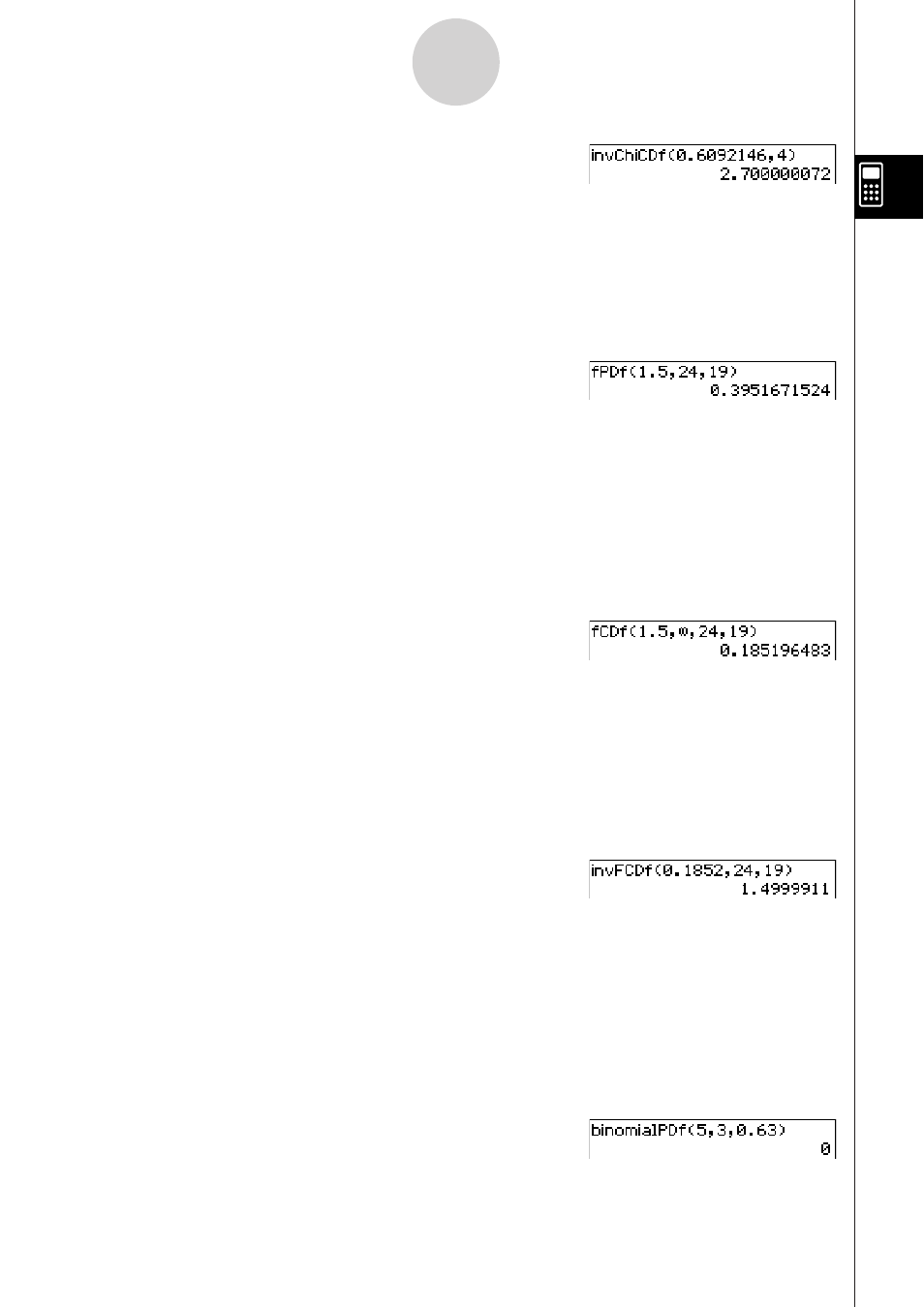
Example: To determine the F probability density when x = 1.5, n : df = 24, d : df = 19
Menu Item: [Action][Distribution][fPDf]
For more information, see “ F Probability Density” on page 7-11-11.
S fCDf
Function: Returns the cumulative probability of an F distribution between a lower bound
and an upper bound.
Syntax: fCDf(lower value, upper value, n : df , d : df [ ) ]
Example: To determine the F distribution probability when lower value = 1.5, upper
value = d, n : df = 24, d : df = 19
Menu Item: [Action][Distribution][fCDf]
For more information, see “ F Cumulative Distribution” on page 7-11-12.
S invFCDf
Function: Returns the lower bound value of an F cumulative distribution probability for
specified values.
Syntax: invFCDf( prob , n : df , d : df [ ) ]
Example: To determine the lower bound value when prob = 0.1852, n : df = 24, d : df = 19
Menu Item: [Action][Inv. Distribution][invFCDf]
For more information, see “Inverse F Cumulative Distribution” on page 7-11-13.
S binomialPDf
Function: Returns the probability in a binomial distribution that the success will occur on
a specified trial.
Syntax: binomialPDf( x , numtrial value, pos [ ) ]
Example: To determine the binomial probability when x = 5, numtrial value = 3,
pos = 0.63
Menu Item: [Action][Distribution][binomialPDf]
For more information, see “Binomial Distribution Probability” on page 7-11-14.