Multiple integrals, Dx x f ), Dydx y x dydx y x da y x – HP 49g+ User Manual
Page 465: Φ φ φ
Page 14-8
The resulting matrix has elements a
11
=
∂
2
φ/∂X
2
= 6., a
22
=
∂
2
φ/∂X
2
= -2.,
and a
12
= a
21
=
∂
2
φ/∂X∂Y = 0. The discriminant, for this critical point s2(1,0)
is
∆ = (∂
2
f/
∂x
2
)
⋅
(
∂
2
f/
∂y
2
)-[
∂
2
f/
∂x∂y]
2
= (6.)(-2.) = -12.0 < 0, indicating a
saddle point.
Multiple integrals
A physical interpretation of an ordinary integral,
∫
b
a
dx
x
f
)
(
, is the area
under the curve y = f(x) and abscissas x = a and x = b. The generalization
to three dimensions of an ordinary integral is a double integral of a function
f(x,y) over a region R on the x-y plane representing the volume of the solid
body contained under the surface f(x,y) above the region R. The region R
can be described as R = {a
∫ ∫
∫ ∫
∫∫
=
=
d
c
y
s
y
r
b
a
x
g
x
f
R
dydx
y
x
dydx
y
x
dA
y
x
)
(
)
(
)
(
)
(
)
,
(
)
,
(
)
,
(
φ
φ
φ
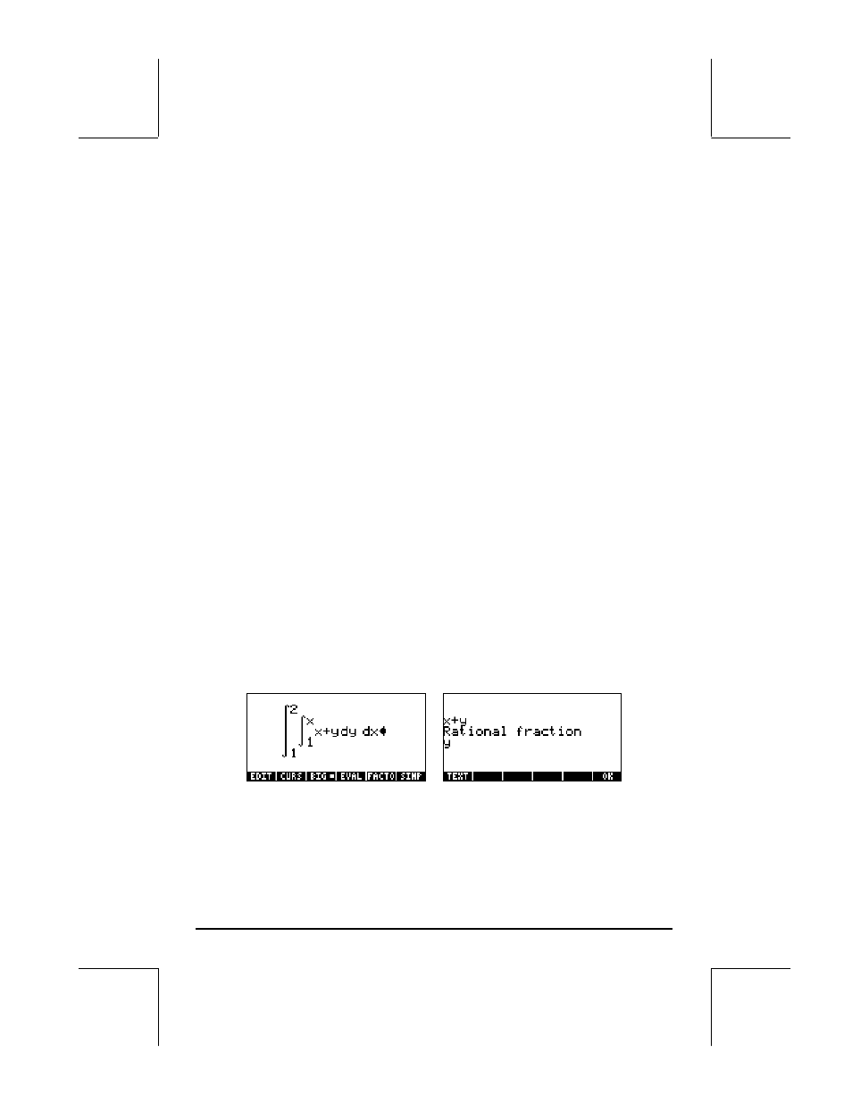
Calculating a double integral in the calculator is straightforward. A double
integral can be built in the Equation Writer (see example in Chapter 2). An
example follows. This double integral is calculated directly in the Equation
Writer by selecting the entire expression and using function
@EVAL. The result
is 3/2. Step-by-step output is possible by setting the Step/Step option in the
CAS MODES screen.