YSI 600LS - User Manual User Manual
Page 72

Sondes
Section 2
YSI Incorporated
Environmental Monitoring Systems Operations Manual
2-66
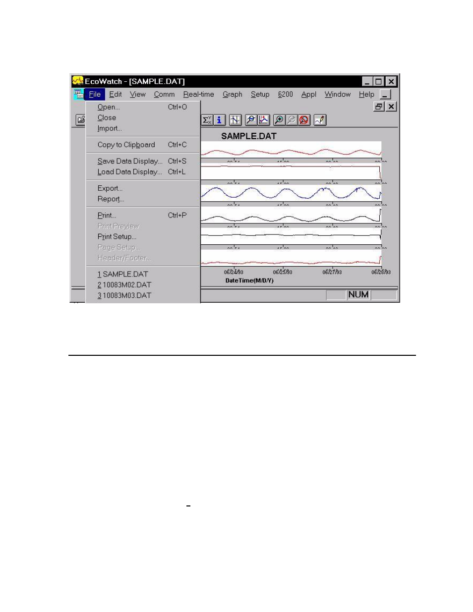
Figure 49 Saving, Exporting, Printing and Related Functions
EXAMPLE OF CUSTOMIZING A SUBSET OF SAMPLE.DAT
To conclude this section we have used a few of the many tools available in EcoWatch to demonstrate how
you might use this powerful plotting and reporting program to express study results. We encourage you to
try some of the tools and learn more about EcoWatch by using the Window‟s Help function, which is
available when the EcoWatch program is running.
Using SAMPLE.DAT we decided that some of the data were not of particular interest, so using top line
menu item Setup, then Parameters, then Add/Remove, we removed ORP and Depth results from the data
set. Note that we have not deleted this information from the file, but rather we are choosing not to display
it. You can always return to this function and add original data back. Under the same Parameters
function, we have selected Attributes and changed the Average Interval from the default 0 to 60. Since
data was collected every 15 minutes, the change to a 60 minute interval helps to smooth out the graph and
average out any short term “noise” events.
Next, we again select Setup, then Graph. From the functions available, we first selected Title Page… and
typed in a name (Clear Lake Study #2) and below that we typed the parameters that are shown in the graph.
Just below Title Page, we clicked on 2 Traces per Graph. This combines adjacent parameters which is
sometimes useful in parameter and event evaluation. For example, in the second graph shown in Figure 50
below, you see that DO concentration and pH seem to track rather closely and change in a diurnal rhythm.
In actuality, when DO levels drop in a natural body of water, CO
2
often builds up forming carbonic acid
which leads to lower pH readings. DO rises again during the day due to photosynthesis, CO
2
then falls and
pH increases again. The final plot after making these changes in shown in Figure 50.
