Metric Halo SpectraFoo Version 1.5 - Manual (Page 37)

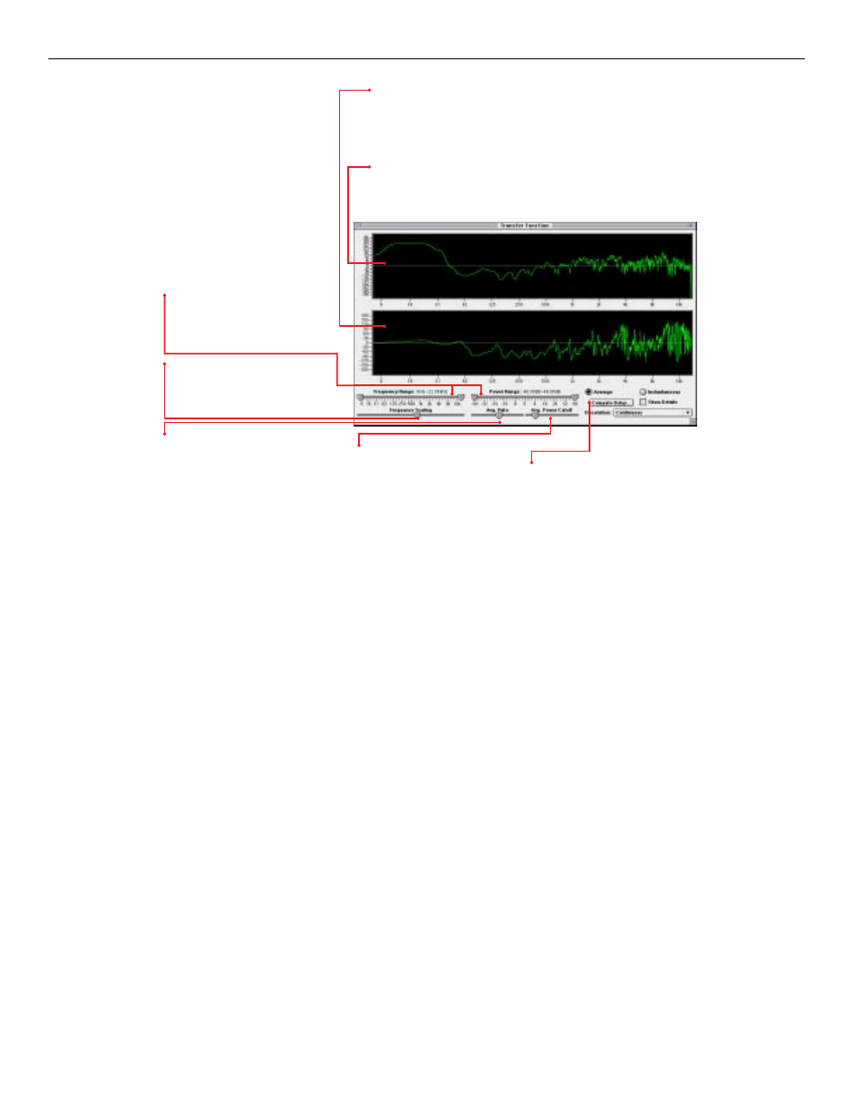
Transfer Function after the measurement has been time-aligned
The Transfer Function’s New Look: v1.5
The parameter controls for the Transfer Function have been moved out of the Transfer Function window and placed
in a details window. This is consistent with the operation of all other SpectraFoo instruments. The Transfer Function
details window is accessed by clicking on the show details button in the Transfer Function window or in the Master
Controls window. In addition, the Transfer Function now has a solo button and an on/off button.
Coherence
The Transfer Function window now has a Coherence trace. Coherence is displayed as a red trace in the power vs.
frequency display. Coherence has a value of 0 when the trace is at the bottom of the display and has a value of 1
when the trace is at the top of the display and varies linearly in between.
Coherence is a measure of how well the response signal correlates with the source signal. When Coherence is at its
maximum value of 1 for a given frequency band, the source and response are perfectly correlated and the Transfer
Function is completely uncontaminated by noise. When Coherence is at its minimum value of 0 for a given frequency
band, there is no correlation between the source and response and the measurement in this frequency band is invalid.
Coherence can be used as a guide to determine which frequency bands are equalizable. Frequency bands for which
Coherence is low cannot be corrected by equalization. Frequency bands for which Coherence is high are equalizable.
Use these sliders to set the frequency and
power ranges used by the display. The
sliders work in exactly the same way as
those found in the Details windows for the
Spectragraph and Spectragram.
The Average Rate Slider allows you to
adjust the time constant of the averaging
process. When the slider is to the far left,
the average value tracks the instantane-
ous measurements quite closely. As the
slider is moved to the right, the average is
computed from longer and longer periods
of the instantaneous signal.
The Average Power Cutoff Slider allows you
to adjust the minimum amount of signal that
needs to be present in each frequency band
of the source signal before the current
measurement is included in the average
for the frequency band. This is the key to
MBM. Adjust this parameter to trade off
between noise rejection and range of fre-
quencies for which average information will
be computed. Choosing wideband source
material gives you the best S/N vs. band-
width tradeoff.
This slider allows you to set the frequen-
cy scaling of the display. When the slider
is all the way to the left, the scaling is
roughly linear. When the slider is all the
way to the right, the scaling is logarithmic.
Compute Delay calculates the delay bet-
ween the left and right channels and opens
a Delay Finder Window to let you com-
pensate for the delay.
This graph shows the amplitude difference between the source and response signals
as a function of frequency. A trace oriented on the zero line indicates that the source
and response signals are the same. For the frequencies where the trace is above
zero, the response signal has more power than the source. For the frequencies where
the trace is below zero, the response has less power than the source.
This graph shows the relative phase of the source and response signals as a func-
tion of frequency. A trace oriented on the zero line indicates that the signals are in
phase. For frequencies where the trace is above zero, the source is delayed from the
response by the indicated number of degrees. For frequencies where the trace is be-
low zero, the response is delayed from the source by the indicated number of de-
grees.
SpectraFooTDM Operation Guide 36