Ocean Optics S1024DW Install User Manual

Page 21

What You Will Need To Do:

1. After placing OOIBase32 into Scope Mode, take a spectrum of the HG-1. Adjust the integration time

until there are several peaks on the screen that are not off-scale.

2. Move the cursor to one of the peaks and carefully position it so that it is at the point of maximum

intensity. Record the pixel number that is displayed in the status bar. Repeat this step for all of the
peaks in your spectrum.

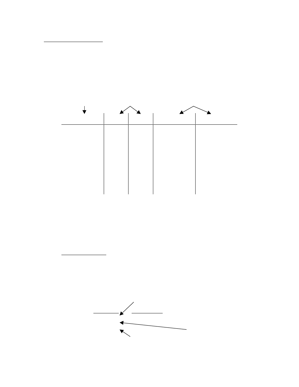
3. Using your spreadsheet, create a table like the one shown below. In the first column, place the exact

wavelength of the spectral lines that you used. In the second column of this worksheet, place the
observed pixel number. In the third column, place the pixel number squared.

Independent

Dependent

Values computed from

Variable

Variables

the regression output

TRUE

Wavelength (nm)

Pixel #

Predicted

Wavelength

Difference

253.65

296.73

302.15

313.16

334.15

365.01

404.66

435.84

546.08

696.54

706.72

727.29

738.40

750.39

105

179

188

206

243

298

368

423

626

921

942

984

1007

1033

11025

32041

35344

42436

59049

88804

135424

178929

391876

848241

887364

968256

1014049

1067089

253.516577

296.979662

302.220703

312.6735

334.037188

365.489132

404.991651

435.615094

545.48766

696.302678

706.638812

727.151647

738.294786

750.814613

0.133422619

-0.249662049

-0.070702657

0.486499891

0.112812248

-0.479132164

-0.331651335

0.224905808

0.592339659

0.237321917

0.081187518

0.138352544

0.105214107

-0.424612735

4. Now you are ready to calculate the wavelength calibration coefficients. In your spreadsheet program,

find the functions to perform linear regressions:

•

in Quattro Pro, look under Tools | Advanced Math

•

in Excel, look under Tools | Data Analysis

5. Select the true wavelength as the dependent variable (Y). Select BOTH the pixel number and pixel

number squared as the independent variables (X). After you execute the regression, an output similar
to the one shown below is obtained.

Regression Statistics

Multiple R

0.999998327

R Square

0.999996654

Adjusted R Square

0.999996096

Standard Error

0.371756477

Observations

intercept

Coefficients

Standard Error

Intercept

190.713498

0.369047536

X Variable 1

0.604451305

0.001684745

X Variable 2

-6.02547E-05

1.41503E-06

first coefficient

second coefficient