Atec Agilent-8510C - Manual (Page 18)

18
Storage
Internal memory
Instrument state: Eight instrument states can be stored
in non-volatile memory via the SAVE menu. They can then
be recalled via the RECALL menu. Instrument states
include all control settings, memory trace data, active list
frequency tables, active calibration coefficients, and custom
display titles. Register 8 is reserved for the power-up state,
which can be defined by the user.
Hardware configurations: One hardware configuration is
stored in active non-volatile memory. This configuration is
not changed at instrument preset. The hardware config-
uration includes all instrument addresses and the multiple
frequency mode parameters.
Data traces: Eight traces of data can be stored in the
trace memories. Traces 1-4 are stored in non-volatile
memory.
Calibration sets: Eight separate calibration sets may be
stored in non-volatile memory. If any 801-point full two-
port calibrations are stored, storage may be limited to as
few as four calibration sets.
Calibration kits: Two calibration kits, including user-
modified kits can be stored in the 8510 internally allo-
cated memory. An internally stored kit is written over
when another calibration kit is loaded in the same data
storage location. Calibration kits can also be stored to
disk.
Internal disk drive: The built-in disk drive can be used
to store and retrieve different types of data on a 3.5 inch
disk. Data files can be stored in either the HP LIF or
MS-DOS
® formats. Diskettes of double sided format or
high density format are recommended.
External disk drive: Data can also be stored on disk
using an external disk drive with command subset SS/80.
Data files are stored in Hewlett-Packard’s standard LIF
or MS-DOS format.
Disk storage memory requirements
Type of Data to be Stored Memory Required (Kbytes)
Calibration set (full two-port, 801 pts) 234
Calibration kit 2
Instrument state 7
Hardware state 0.5
Machine dump 400
Data data (201 pts)
1 S-parameter 5.5
4 S-parameters 20
Data formatted, raw or memory (201 pts) 5.5
User display 33
Time domain (Option 010)
Description
With the time domain option, data from transmission or
reflection measurements is converted from the frequency
domain to the time domain using the inverse Fourier
transform and presented on the CRT display. The time
domain response shows the measured parameter value
versus time. Markers may also be displayed in electrical
length (or physical length if the relative propagation
velocity is entered).
Time stimulus modes
Two types of time domain stimulus waveforms can be sim-
ulated during the transformation — a step and an
impulse. Although these waveforms are generated mathe-
matically with the inverse FFT, the results for linear cir-
cuits are the same as would be obtained if the actual time
waveforms had been applied and measured.
Low pass step: This stimulus, similar to a traditional
Time Domain Reflectometer (TDR) waveform, is used to
measure low pass devices. Transforming to time low pass
requires a sweep over a harmonic set of frequencies includ-
ing an extrapolated DC value. The step response is typi-
cally used for reflection measurements only. The low pass
step waveform displays a different response for each type
of impedance (R, L, C), giving useful information about the
discontinuities being measured.
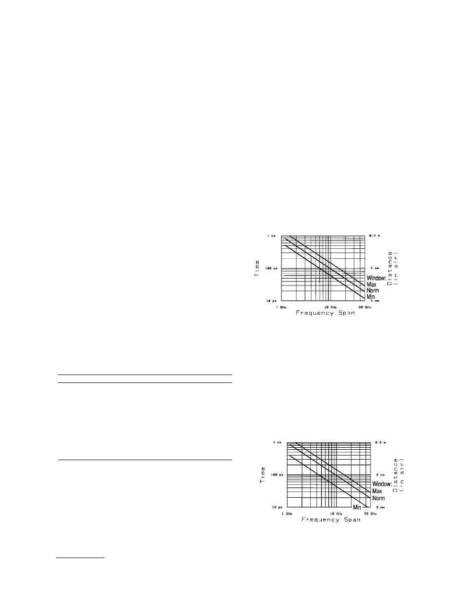
Response resolution
1 : In low pass step mode, response
resolution is determined by the step rise time (10% to
90%) of the time stimulus. This depends on both the
frequency span and the window used (see Windows):
Low pass impulse: This stimulus is also used to
measure low pass devices, and is the mathematical
derivative of the low pass step response. Transforming to
time low pass requires a sweep over a harmonic set of fre-
quencies including an extrapolated DC value. The time
domain response shows changes in the parameter value
versus time. The impulse response can be used for reflec-
tion (fault location) or transmission measurements.
Response resolution
1 : In low pass impulse mode,
response resolution is defined by the 50% impulse width of
the time stimulus. This depends on both the frequency
span and the window used (see Windows):
1. Response resolution is the ability to resolve two closely spaced responses of equal magnitude. For example, in time
impulse response, two equal responses that are separated in time by less than one impulse width cannot be
resolved as two separate responses.