d&b TI 385 d&b Line array design - Manual (Page 40)

Aligning a L/R subwoofer setup
The delay alignment tool can also be used to align L/R
ground stacked subwoofers to any other source. Set the
number of subwoofer sources to 1. Now only the center
source is active. Enter the x and y coordinates of the left
ground stack and proceed as before.
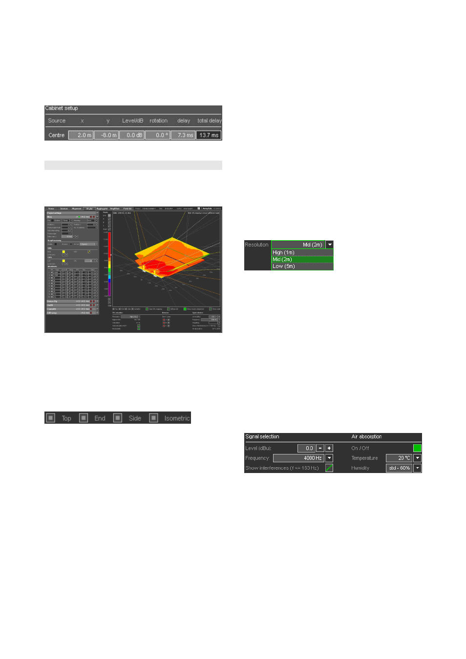
10.12 3D plot page
ArrayCalc offers the possibility to calculate an SPL mapping
including all sources in the project on all defined listening
planes for a selectable third octave frequency band.
ArrayCalc, 3D plot
The left side of the page contains a fully operable copy of
the project, room and source settings of the project.
The calculation results are displayed in a zoomable, mouse
controlled 3D diagram that is fully rotatable.
Preset views
Directly underneath the diagram area, you can choose
between different standard views: "Top" - view from above
onto the x-y plane, "End" - view from the end onto the y-z
plane, "Side" - view from the house left side onto the x-z
plane and a standard 30°/30° "Isometric" view. The
preset views always affect the diagram situated directly
above them.
In addition, you can define any other view by clicking and
holding down the left mouse button in the diagram when
moving the mouse. An up/down movement rotates the
viewport around the x-axis, a left/right movement rotates it
around the y-axis.
Holding down the right mouse button while moving
left/right rotates the viewport around the z-axis. The
distance between the click position and the rotational axis
defines the leverage of the movement.
Turning the mouse wheel zooms in and out.
You can also move the diagram by holding down the CTRL
key (Apple key for Macintosh) while clicking in the diagram
and holding down the left mouse button when moving the
mouse.
If you are completely lost, simply click one of the preset
views or double-click into the diagram. This will restore the
last preset view selected.
Show sources / show source dispersion
When the Show sources switch is enabled, 3D rendered
drawings of all sources are displayed. As usual, the
selected source is highlighted.
When the Show source dispersion switch is enabled, the
main axis of the first TOP cabinet of each array as well as
the nominal dispersion axes of the first and the last TOP
cabinets of each array are displayed in the diagram. For
point sources, the main axis of each cabinet is displayed.
Spatial resolution of the SPL mapping
Mapping resolution
The spatial resolution of the mapping calculation in the 3D
plot can be selected underneath the diagram. Possible
settings are High (1 m) / Mid (2 m) / Low (5 m). Between
each of them, the time for a full calculation increases by a
factor of 4. A resolution of 2 m is used as default setting.
Be aware that high resolution mapping calculations of large
venues (arena or stadium) using many large arrays can
easily exceed 15 minutes of calculation time and will
require a lot of RAM memory!
For detailed calculations of particular areas only the
relevant listening planes may be switched on in the Room
settings menu. This improves calculation time and ensures a
maximum sized display of the planes.
Signal selection and SPL summation method
You can select the simulated frequency range in standard
third octave bands.
For frequency bands of 163 Hz and below you can use
complex SPL summation as an option thus showing
interferences. (SPL calculation within each array is always
based on complex summation). Higher frequencies are
always displayed as an energy sum.
To display interferences correctly and totally, the spatial
resolution of the mapping has to be in the range of half the
wavelength of the simulated frequency. The 163 Hz band is
able to fulfill this requirement for a minimum resolution of
1 m.
TI 385 (6.0 EN) d&b Line array design, ArrayCalc V8.x Page 40 of 54