d&b TI 385 d&b Line array design - Manual (Page 37)

Export/import of SUB array settings
You can export defined SUB array settings to an ArrayCalc
description file (*.dbesa). This file including the exported
SUB array settings can then be imported in other projects or
in the same project again, for example for comparative
purposes.
To use the SUB array export/import function, right-click in
the SUB array dialog to activate the context menu or select
'Export source/Import source' from the Sources menu.
10.10.7 Mixed arrays of J-, V-SUBs and J-INFRAs
In general, a SUB array should always be set up using
identical systems for all positions in order to obtain a
predictable and frequency consistent total behavior.
However, it is possible to build a SUB array consisting of
source positions with J-SUBs, V-SUBs or J-INFRAs. The
dispersion characteristics of these subwoofer types have
been closely matched across their entire frequency ranges
and the full spheres to enable a combined operation.
In this case, a default ratio of 2 x V-SUBs to 1 x J-SUB is set
in order to balance the SPL/headroom.
A setup consisting of alternating positions of 3 x J-SUBs and
2 x J-INFRAs is most beneficial. The same applies to a
setup consisting of alternating positions of 2 x V-SUBs and
1 x J-INFRA. In such a combination, the J-INFRA subwoofers
can provide all the extended frequency range on the very
low end with sufficient headroom. However, it is important
to match the upper frequency extension.
If you have selected a mixed array of J/V-SUB and J-INFRA
subwoofers in the SUB systems drop-down list, the cabinet
types listed in the Cabinet setup section are displayed in a
list box from which you can select the system for each
position.
The bandwidth selection switches (Switch 1) of the two
systems work in reverse, i.e the J-SUB has an "INFRA" (the
V-SUB a 100 Hz) switch lowering the upper frequency
extension when "on", while the J-INFRA has a "70 Hz"
switch rising the upper frequency extension when "on".
Consequently, they have to be combined and are mutually
exclusive. When you activate one, the other one is
disabled. Their proper use is controlled by the "hip/hop"
selector.
10.10.8 Dispersion displays
The following displays help to evaluate the performance of
the array.
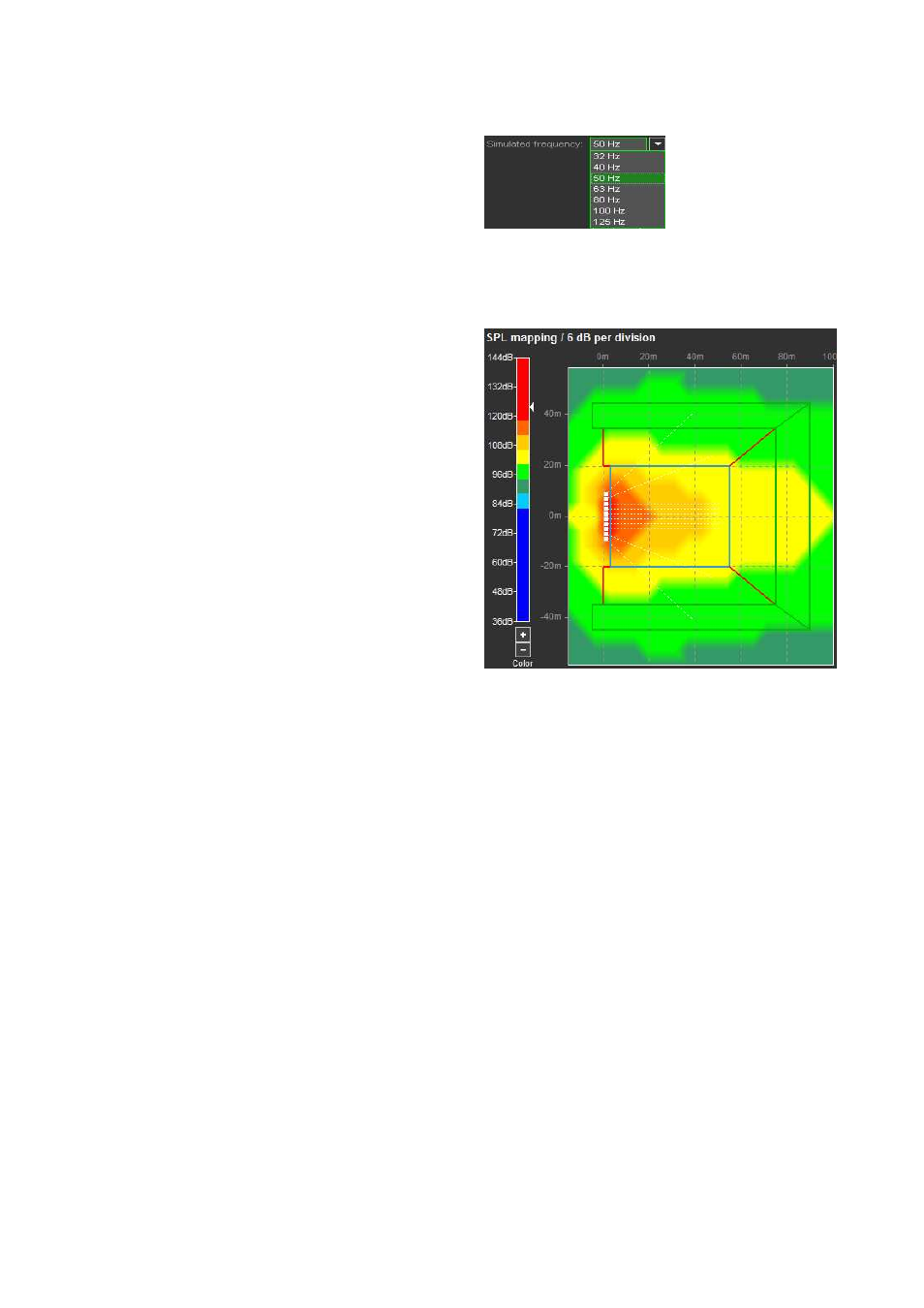
Mapping diagram
Select the simulation frequency.
Consider and compare all relevant frequencies within the
system´s operating bandwidth. Each colored isobar
represents a drop in level by 6 dB. Place the mouse onto
the drop-down list and use the wheel to quickly change
between the frequencies.
Mapping diagram with color scale
Color scale
The color scale for the SPL mapping has a fixed 6 dB per
division resolution. The color scale window displayed can
be set according to the calculation results. This is done by
either clicking the +/-- buttons underneath the scale or
using the mouse wheel while the mouse pointer is on the
scale. The small arrow to the right of the scale indicates the
highest SPL value calculated for the plot.
The color scale does not rescale automatically. This enables
you to quickly notice the result of any change in the setup
while optimizing the project.
Polar diagram
Polar diagrams visualize the far field behavior of the array,
i.e. the dispersion pattern at a distance which is much larger
than the array dimensions.
Although this distance might often extend beyond the actual
audience area, the polar diagram provides helpful
information about the consistency of the dispersion patterns
for different frequency bands displayed in a single plot.
Third-octave frequency bands between 32 Hz and 100 Hz
can be selected, as well as the octave average at 40 Hz
and 80 Hz.
TI 385 (6.0 EN) d&b Line array design, ArrayCalc V8.x Page 37 of 54