Best fit line, Procedure, Analysis – PASCO AP-8215A Gravitational Torsion Balance User Manual
Page 17

®
M o d e l N o . A P - 8 2 1 5 A
M E T H O D I I I : M e a s u r e m e n t b y A c c e l e r a t i o n
13
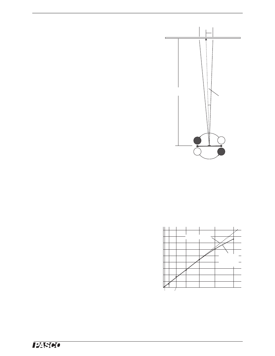
The acceleration is measured by observing the displacement of the
light spot on the screen. If, as is shown in Figiure 19:
s = the linear displacement of the small masses,
d = the distance from the center of mass of the small masses to
the axis of rotation of the torsion balance,
S= the displacement of the light spot on the screen, and
L= the distance of the scale from the mirror of the balance,
then, taking into account the doubling of the angle on reflection,
Using the equation of motion for an object with a constant acceler-
ation (x = 1/2 at
2
), the acceleration can be calculated:
By monitoring the motion of the light spot over time, the accelera-
tion can be determined using equation 3.6, and the gravitational
constant can then be determined using equation 3.4.
Procedure
1. Begin the experiment by completing steps 1–3 of the procedure detailed in Method I.
2. Immediately after rotating the swivel support, observe the light spot. Record the position of the light spot (S)
and the time (t) every 15 seconds for about two minutes.
Analysis
1. Construct a graph of light spot displacement (
S = S -
S
1
) versus time squared (t
2
), with t
2
on the horizontal
axis (Figure 20). Draw a best-fit line through the
observed data points over the first minute of observa-
tion.
2. Determine the slope of your best-fit line.
3. Use equations 3.4 and 3.6 to determine the gravita-
tional constant.
4. The value calculated in step 3 is subject to a system-
atic error. The small sphere is attracted not only to its
neighboring large sphere, but also to the more distant
large sphere, although with a much smaller force. Use
the procedure detailed in Method I (Analysis, step 3)
to correct for this force.
S
1
S
2
ΔS
2
2
θ
L
Figure 19: Source of data for
calculations in Method III
S
s 2L
d
------
3.5
=
a
0
2
s
t
2
---------
Sd
t
2
L
----------
3.6
=
=
Δ
S
0
1
2
3
4
5
6
7
8
9
225
2025
900
3600
5625
8100
11025
t
2
(sec
2
)
Best Fit Line
Curve
Through
Data
Figure 20: Sample data and best-fit line
