HP 15c - Manual (Page 49)

Section 2: Working with f 49
Although the branch for u=1 adds four steps to your subroutine, integration near x = 0
becomes more accurate.
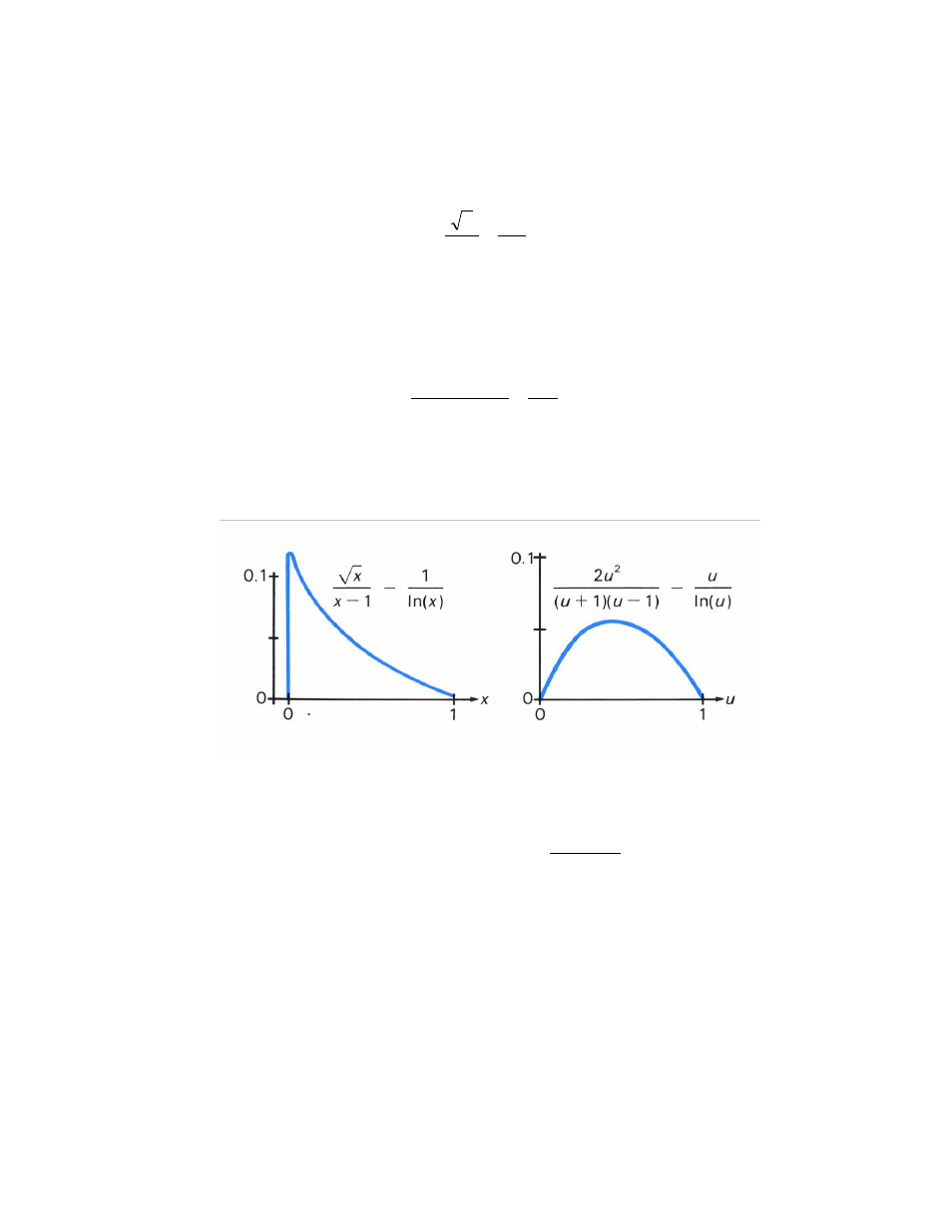
As a second example, consider the integral









1
0 ln
1
1
dx
x x
x
.
The derivative of the integrand approaches ∞ as x approaches 0, as shown in the illustration
below. By substituting x = u
2
, the function becomes more well behaved, as shown in the
second illustration. This integral is easily evaluated:








 
1
0
2
ln ) 1 )( 1 (
2
du
u
u
u u
u
.
Don't replace (u + 1)(u − 1) by (u
2
− 1) because as u approaches 1, the second expression
loses to roundoff half of its significant digits and introduces to the integrand's graph a spike
near u = 1.
As another example, consider a function whose graph has a long tail that stretches out many,
many times as far as the main "body" (where the graph is interesting)-a function like
2
) ( x e x f
 
or
10 2 10
1
) (
 

x
x g .
Thin tails, like that of f(x), can be truncated without greatly degrading the accuracy or speed
of integration. But g(x) has too wide a tail to ignore when calculating


t
t
dx x g ) (
if t is large.
For such functions, a substitution like x = a + b tan u works well, where a lies within the
graph's main "body" and b is roughly its width. Doing this for f(x) from above with a = 0 and
b = 1 gives