Dwyer AFG - Manual (Page 5)

Calibration on Site:
To achieve the best possible accuracy, the AFG Flow Grids must
be calibrated on site and the following method of site calibration
and subsequent calculation is advised.
Any valid method of determining the volume flow rate may be used
in establishing the flow rate to differential pressure characteristic.
The following method and theory applies to the use of Pitot static
tubes, as the primary means of determining volume flow rate by
the velocity traverse technique.
To calibrate an AFG Flow Grid:
1. Install the AFG Flow Grid as described (See installation pages 2
& 3) and connect to a suitable manometer.
2. Prepare holes in the duct wall upstream of the AFG Flow Grid
for the Pitot static tube traverse to give an adequate survey of the
duct velocity pattern and mean duct velocity.
3. Operate the system to give a typical flow rate through the Flow
Grid and take records of Pitot static tube traverse readings and the
Flow Grid differential pressure readings.
4. If possible, arrange the system flow rate to be changed to give
additional sets of readings covering the range over which the sys-
tem is intended to be used.
5. The theory of the AFG Flow Grid for normal atmosphere condi-
tions is shown on page 4.
(Δp)/(Pv)= M (See page 4).
Measure the ambient temperature ‘t’, the ambient barometric
pressure ‘B’ and the duct static pressure Ps. Calculate the cor-
rection factor CF in the appropriate units.
Hence calculate the flow constant ‘K’ for each set of readings
taken.
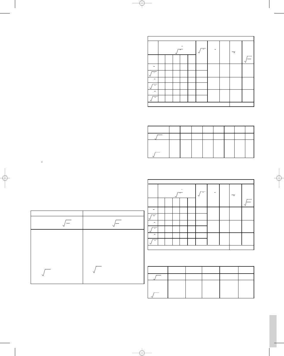
Table 5: Calculating Flow Constant K
6. Suggested format for results using worked examples:
Metric Units (example- using AFG Flow Grid in duct size 250 mm
x 500 mm)
Table 6: Example: K Factor Calculation (Metric)
Table 7: Graph Plotting Information Derived from Traverse
Data (metric)
Imperial Units (example- using AFG Flow Grid in duct size 10” x
20”)
Table 8: Example: K Factor Calculation (Imperial)
Table 9: Graph Plotting Information Derived from Traverse
Data (Imperial)
(see Fig. 17 for Graph)
page 5
Where =
Δp = X Flowgrid differential pressure
M = X Flow grid magnification factor
Pv = duct mean velocity pressure Pa
A = cross section area of duct m
2
CF = correction factor
Take the average K
1 and plot the
curve of Q v Δp
Where
Q = K
1 Δp
Q = volume flowrate m 3 /s
Δp = X Flowgrid differential pressure in. wg.
M = X Flowgrid magnification factor
Pv = duct mean velocity pressure wg
A = cross section area of duct ft
2
CF = correction factor
Q = K 1 Δp
Q = volume flowrate ft 3 /min
K 1 = A x 1.291 CF
M
K 1 = A x 4005 CF
M
SI Units Imperial Units
1
250
15.81
96
9.80
48
6.93
2
230
15.17
92
9.59
46
6.78
3
260
16.12
99
9.95
47
6.86
4
240
15.49
96
9.80
51
7.14
5
212
14.56
90
9.49
45
6.71
Reading
No.
Pitot Tube Traverse
Readings Pv Pa
& Pv
Average
of
Pv
Flow-
grid
Diff
Δp
Mag-
Factor
Δp = M
Pv
PITOT STATIC TUBE TRAVERSE DATA
Average
of
Pv
Flow
Constant
K1 =
Ax1.291
CF
M
Pv
Pv
Pv
Pv
Pv
Pv
15.43
9.73
6.88
238.08
94.67
47.33
514.2
199.8
98.1
2.160
2.110
2.072
0.1095
0.1108
0.1118
DUCT AREA A = 250 X 500 mm = 0.125 m 2 AVERAGE k 1 = 0.1107
1
0.95
0.975
0.48
0.693
0.23
0.480
2
0.99
0.995
0.50
0.707
0.25
0.50
3
1.03
1.015
0.52
0.721
0.25
0.50
4
1.06
1.030
0.53
0.728
0.24
0.49
5
0.99
0.996
0.49
0.70
0.22
0.469
Reading
No.
Pitot Tube Traverse
Readings Pv Pa
& Pv
Average
of
Pv
Flow-
grid
Diff
Δp
Mag-
Factor
Δp = M
Pv
PITOT STATIC TUBE TRAVERSE DATA
Average
of
Pv
Flow
Constant
K1 =
Ax4005
CF
M
Pv
Pv
Pv
Pv
Pv
Pv
1.002
0.710
0.488
1.004
0.504
0.238
2.169
1.063
0.493
2.160
2.110
2.072
3781
3828
3863
DUCT AREA A = 10˝ X 20˝ = 1.388 ft 2 AVERAGE k 1 = 3824
25
5
0.553
50
7.07
0.783
100
10
1.107
200
14.14
1.565
300
17.32
1.917
400
20.0
2.214
500
22.36
2.475
600
24.43
2.704
MX Flow Grid
Diff Δp Pa
Δp
Vol Flow
Rate
Q = K 1
ΔpM 3 /s
0.5
0.707
2703
1.0
1.0
3824
1.5
1.225
4684
2.0
1.414
5408
2.5
1.581
6046
MX Flow Grid
Diff Δp Pa
Δp
Vol Flow
Rate
Q = K 1
Δpft 3 /min
AFG iom1 1/3/06 2:00 PM Page 5