Normal and inverse–normal distributions, Dx e x q – HP 33s User Manual
Page 271

Statistics
Programs
16–11
Logarithmic
Exponential
Power
To start:
X
L
X
E
X
P
R
0.9965 0.9945 0.9959
M
–139.0088 51.1312 8.9730
B
65.8446 0.0177 0.6640
Y
(
yˆ
when X=37)
98.7508 98.5870 98.6845
X
(
xˆ
when Y=101)
38.2857 38.3628 38.3151
Normal and Inverse–Normal Distributions
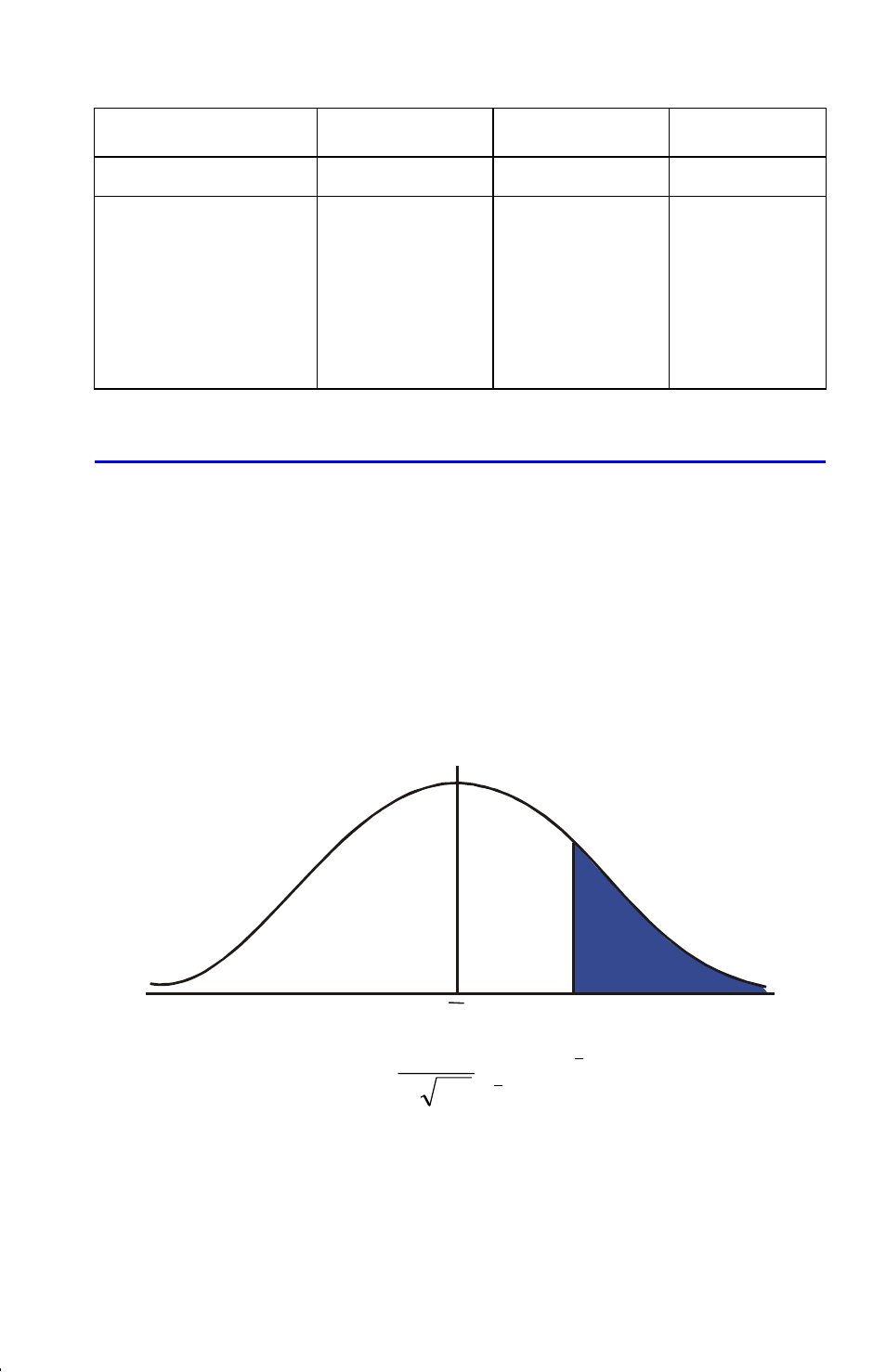
Normal distribution is frequently used to model the behavior of random variation
about a mean. This model assumes that the sample distribution is symmetric about
the mean, M, with a standard deviation, S, and approximates the shape of the
bell–shaped curve shown below. Given a value x, this program calculates the
probability that a random selection from the sample data will have a higher value.
This is known as the upper tail area, Q(x). This program also provides the inverse:
given a value Q(x), the program calculates the corresponding value x.
x
y
"Upper tail"
area
x
Q [x]
³
ч
ч
−
−
−
=
x
x
x
x
dx
e
x
Q
2
)
)
((
2
2
1
5
.
0
)
(
σ
π
σ
This program uses the built–in integration feature of the HP 33s to integrate the
equation of the normal frequency curve. The inverse is obtained using Newton's
method to iteratively search for a value of x which yields the given probability
Q(x)
.
