Thermo Fisher Scientific Ion Selective Electrodes Sodium - Manual (Page 6)

Sodium Electrode Instruction Manual
4
TABLE 1: Concentration Unit Conversion Factors
ppm
Na
+
moles/liter Na
+
229.90 1.0 x 10-
2
22.99 1.0 x 10-
3
2.30 1.0 x 10-
4
MEASUREMENT PROCEDURE
Direct Measurement
Direct measurement is a simple procedure for measuring a large number of samples. A single meter
reading is all that is required for each sample. The ionic strength of samples and standards should
be made the same by adjustment with ISA for all sodium solutions. The temperature of both sample
solution and of standard solutions should be the same.
Direct Measurement of Sodium (using a pH/mV meter)
1. By serial dilution of the 0.1 M or 1,000 ppm standards, prepare 10-
2
M, 10-
3
M, and 10-
4
M
or 100 and 10 ppm sodium standards. Add 2 ml of ISA per 100 ml of standard. Prepare
standards with a composition similar to the samples if the samples have an ionic strength
above 0.1M.
2.
Place the most dilute solution (10-
4
M or 10 ppm) on the magnetic stirrer and begin
stirring at a constant rate. After assuring that the meter is in the mV mode, lower the
electrode tips into the solution. When the reading has stabilized, record the mV reading.
3.
Place the mid-range solution (10-
3
M or 100 ppm) on the magnetic stirrer and begin
stirring. After rinsing the electrodes with electrode rinse solution, blot dry and immerse
the electrode tips in the solution. When the reading has stabilized, record the mV reading.
4.
Place the most concentrated solution (10-
2
M or 1,000 ppm) on the magnetic stirrer and
begin stirring. After rinsing the electrodes with electrode rinse solution, blot dry and
immerse the electrode tips in the solution. When the reading has stabilized, record the
mV reading.
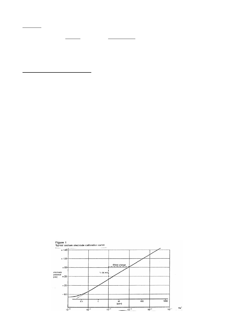
5. Using the semi-logarithmic graph paper, plot the mV reading (linear axis) against the
concentration (log axis). Extrapolate the curve down to about 5.0X10-
5
M. For
measurements below this level, follow the instructions for low-level measurement. A
typical calibration curve can be found in Figure 1.