Yokogawa JUXTA VJXS - Manual (Page 4)

4 IM 77J01X11-01E 2nd Edition Nov 30,2005-00
6.3 VJXS-C Dead Time Computation
This computing unit stores the input values (X) sampled at intervals of
one-fortieth of the dead time (L) into 40 buffers in order and outputs
data (output-1 = Y1, output-2 = Y2) after the dead time has elapsed.
Minimum sampling time is the set computation cycle. Therefore,
when the dead time is set shorter, the number of samplings is less
than 40. The output between samplings is smoothed out by interpola-
tion.
However, for the dead times of 3, 2 and 1 second, the number of sam-
plings is 30, 20, and 10, respectively (when the computation cycle is
100ms). When using a first-order lag filter for input (X), set the first-or-
der lag time constant (T).
Set the dead time (L) at % value in H02: CONST. The value of 0 to
100.0% corresponds to that of 0 to 1000 seconds. For example, enter
“6” in H02 to set 60 seconds.
● Setting range of dead time:
0 to 320000 seconds (about 3.7 days) with 4 significant digits;
minimum unit is 1 second (however, 0.1 second for a setting of
4 seconds or shorter). 0.0 to 32000% can be set in H02.
( e.g. 12345% unacceptable, 12340% acceptable)
● Setting accuracy of dead time: (
±
5.0% of set value)
±
1 second.
Set the first-order lag time constant (T) at % value in H01: CONST.
The value of 0 to 100% corresponds to that of 0 to 100 seconds.
● Setting range of first-order lag time constant:
1.0 to 799.0 seconds; the value of 1.0 to 799.0% corresponds to
that of 1.0 to 799.0 seconds; minimum unit is 0.1 second.
However, when not using the first-order lag function, set 0 sec-
ond.
● Setting accuracy of first-order lag time constant :
(
±
5.0% of set value)
±
1 second
Y1=Y2= X
e -L[s]
1+T[s]
e.g. 0%
→
100% step input
Input
Output
L
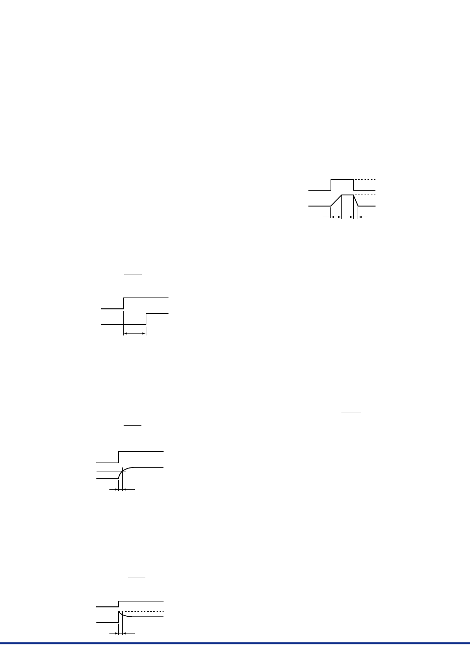
6.4 VJXS-D First-order Lag Computation
This computing unit provides a first-order lag computation on input (X)
with a time constant (T) and outputs the result (output-1 = Y1, output-
2 = Y2). Set the time constant (T) at % value in H01: CONST. The
value of 0 to 100% corresponds to that of 0 to 100 seconds.
● Setting range of first-order lag time constant:
1.0 to 799.0 seconds; minimum unit is 0.1 second.
● Setting accuracy of first-order lag time constant :
(
± 5.0% of set value) ± 1 second
Y1=Y2= X
1
1+T[s]
e.g. 0% → 100% step input
Input 0%
63.2%
100%
100%
Output 0%
T
6.5 VJXS-E First-order Lead Computation
This computing unit provides a first-order lead computation on input
(X) with a time constant (T) and outputs the result (output-1 = Y1, out-
put-2 = Y2). Set the time constant (T) at % value in H01: CONST. The
value of 0 to 100% corresponds to that of 0 to 100 seconds.
● Setting range of first-order lead time constant:
1.0 to 799.0 seconds; minimum unit is 0.1 second.
● Setting accuracy of first-order lead time constant :
(
±
5.0% of set value)
±
1 second
Y1=Y2= (1+ ) X
T[s]
1+T[s]
e.g. 0%
→
50% step input
Input 0%
68.4%
50%
100%
50%
Output 0%
T
6.6 VJXS-F Uniform-speed Response (Velocity
Limiter)
This computing unit limit the input (X) velocity at the ascending veloc-
ity limit for a positive change and the descending velocity limit for a
negative change, and outputs the limited value (output-1 = Y1, output-
2 = Y2). When the input velocity (slope) is no more than the limit
value, the unit outputs the input as is.
Set the ascending velocity limit at % value in H01:CONST, and the
descending velocity limit at % value in H02:CONST. The value of 0 to
100.0% corresponds to that of 0 to 100.0%/minute.
● Setting range of velocity limit:
0.1 to 699.9%/minute; minimum unit is 0.1%/minute.
Setting the limit at 700.0%/minute or above does not limit the in-
put, so the unit simply outputs the input as is (i.e., works as an
open limit function).
● Setting accuracy of velocity limit:
(
±
5.0% of set value)
±
0.1%/minute
e.g. 0% → 100% → 0% step input
Input 0%
100%
100%
Output 0%
Ascending velocity limit
(%/minute)
Descending velocity limit
(%/minute)
6.7 VJXS-G Limiter
This computing unit serves as an ordinary computing unit as long as
the input (X) is within the upper and lower limits. When the input ex-
ceeds the limit, the unit outputs the signal that corresponds to the limit
value (output-1 = Y1, output-2 = Y2).
Set the upper limit at % value in H01:CONST, and the lower limit at %
value in H02:CONST.
● Setting range of upper and lower limits:
−
6.0% to 106.0%; minimum unit is 0.01%.
However, if the setting is made so that the upper limit < lower limit,
the unit outputs the upper limit.
6.8 VJXS-H Velocity Computation
This computing unit calculates the input velocity by subtracting the in-
put of the last velocity computation (X
L
) from the present input (X). The
unit then adds a 50% bias to one-half of the obtained velocity and out-
puts the result (output-1 = Y1, output-2 = Y2). The output results is
50% when the input is not changed, 50% or more when the input in-
creases (100% for X
−
X
L
= 100%), and 50% or less when the input de-
creases (0% for X
−
X
L
=
−
100%). When using a first-order lag filter for
input (X), set the first-order lag time constant (T).
Y1=Y2= +50%
X–X
L
2
Set the velocity computation time (L) at % value in H02: CONST. The
value of 0.0 to 100.0% corresponds to that of 0 to 1000 seconds. For
example, enter “6” in H02 to set 60 seconds.
● Setting range of velocity computation time:
0 to 320000 seconds (about 3.7 days) with 4 significant digits;
minimum unit is 1 second (however, 0.1 second for a setting of
4 seconds or shorter). 0.0 to 32000% can be set in H02.
( e.g. 12345% unacceptable, 12340% acceptable)
● Setting accuracy of velocity computation time: (
±
5.0% of set
value)
±
1 second
Set the first-order lag time constant (T) at % value in H01: CONST.
The value of 0 to 100% corresponds to that of 0 to 100 seconds.
● Setting range of first-order lag time constant:
1.0 to 799.0 seconds; minimum unit is 0.1 second.
However, when not using the first-order lag function, set 0 sec-
ond.
● Setting accuracy of first-order lag time constant :
(
±
5.0% of set value)
±
1 second