EdgeWare FastBreak Standard Version 6.2 - Manual (Page 84)

84
Appendix A - Technical Discussion
Curve Fitting
FastBreak uses three different types of curve fits: Least Squares Linear, Power (called
non-linear on menu), and Quadratic.
Linear is the most common curve fit and has the form: y = a
1
x + a
0
Where:
x : is the independent variable (in our case, days)
y : is the dependent variable (in our case the normalized NAV)
a : is a constant
The slope is the rate of change of y with respect to x. For this equation the slope is a
1
(a
constant value)
The Quadratic equation has the form: y = a
2
x
2
+a
1
x + a
0
The slope is: 2 a
2
x+ a
1
(slope varies with x)
The Power equation has the form: y = a x
b
b : is a constant
The slope is: abx
b-1
Again, the slope varies with x
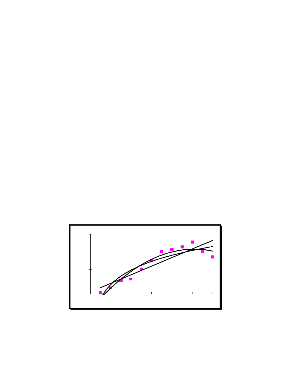
How do these equations look when plotted?
Normalized Price Data
y = 0.0037x + 1.0009
y = 0.9947x 0.0178
y = -0.0005x 2 + 0.0101x + 0.9858
1.00
1.01
1.02
1.03
1.04
1.05
0 2 4 6 8 10 12
T rading Days
N
A
V
Each equation has a somewhat different fit to the data. The NAV is normalized in Fast-
Break by dividing the NAV of each trading day by the NAV of the first trading day at the
start of the ranking period.