Yokogawa JUXTA MXS - Manual (Page 5)

5 IM 77J04X11-01E 2nd Edition Nov 30,2005-00
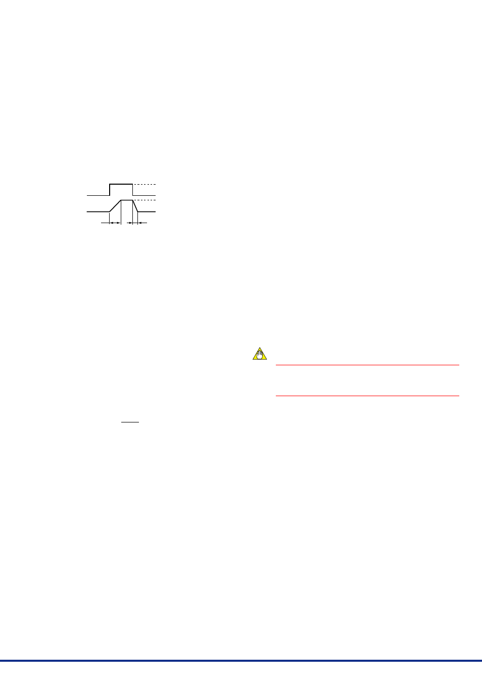
6.6 MXS-F Uniform-speed Response (Velocity
Limiter)
This computing unit limit the input (X) velocity at the ascending veloc-
ity limit for a positive change and the descending velocity limit for a
negative change, and outputs the limited value (output-1 = Y1, output-
2 = Y2). When the input velocity (slope) is no more than the limit
value, the unit outputs the input as is.
Set the ascending velocity limit at % value in H01:CONST, and the
descending velocity limit at % value in H02:CONST. The value of 0 to
100.0% corresponds to that of 0 to 100.0%/minute.
● Setting range of velocity limit:
0.1 to 699.9%/minute; minimum unit is 0.1%/minute.
Setting the limit at 700.0%/minute or above does not limit the in-
put, so the unit simply outputs the input as is (i.e., works as an
open limit function).
● Setting accuracy of velocity limit:
(
±
5.0% of set value)
±
0.1%/minute
e.g. 0% → 100% → 0% step input
Input 0%
100%
100%
Output 0%
Ascending velocity limit
(%/minute)
Descending velocity limit
(%/minute)
6.7 MXS-G Limiter
This computing unit serves as an ordinary computing unit as long as
the input (X) is within the upper and lower limits. When the input ex-
ceeds the limit, the unit outputs the signal that corresponds to the limit
value (output-1 = Y1, output-2 = Y2).
Set the upper limit at % value in H01:CONST, and the lower limit at %
value in H02:CONST.
● Setting range of upper and lower limits:
−
6.0% to 106.0%; minimum unit is 0.01%.
However, if the setting is made so that the upper limit < lower limit,
the unit outputs the upper limit.
6.8 MXS-H Velocity Computation
This computing unit calculates the input velocity by subtracting the in-
put of the last velocity computation (X
L
) from the present input (X). The
unit then adds a 50% bias to one-half of the obtained velocity and out-
puts the result (output-1 = Y1, output-2 = Y2). The output results is
50% when the input is not changed, 50% or more when the input in-
creases (100% for X
−
X
L
= 100%), and 50% or less when the input de-
creases (0% for X
−
X
L
=
−
100%). When using a first-order lag filter for
input (X), set the first-order lag time constant (T).
Y1=Y2= +50%
X–X
L
2
Set the velocity computation time (L) at % value in H02: CONST. The
value of 0.0 to 100.0% corresponds to that of 0 to 1000 seconds. For
example, enter “6” in H02 to set 60 seconds.
● Setting range of velocity computation time:
0 to 320000 seconds (about 3.7 days) with 4 significant digits;
minimum unit is 1 second (however, 0.1 second for a setting of
4 seconds or shorter). 0.0 to 32000% can be set in H02.
( e.g. 12345% unacceptable, 12340% acceptable)
● Setting accuracy of velocity computation time: (
±
5.0%of set
value)
±
1 second
Set the first-order lag time constant (T) at % value in H01: CONST.
The value of 0 to 100% corresponds to that of 0 to 100 seconds.
● Setting range of first-order lag time constant:
1.0 to 799.0 seconds; minimum unit is 0.1 second.
However, when not using the first-order lag function, set 0 sec-
ond.
● Setting accuracy of first-order lag time constant :
(
±
5.0% of set value)
±
1 second
6.9 MXS-J Linearizer (Optionally-set Line-segment
Function)
This computing unit gives an optional relationship between the input
(X) and output (output-1 = Y1, ouput-2 = Y2) signals using an option-
ally-set line-segment function. The line-segment function has 21
breakpoints, which each gives an input-output relationship as a per-
centage (%).
Set the number of line segments by 1 to 20.
Set the input (X) at % value in H01:CONST to H21:CONST, and the
output (Y) at % value in H22:CONST to H42:CONST.
● Setting condition of breakpoints:
For input:
−
6.0 Ϲ X
0
(H01) to X
20
(H21) Ϲ 106.0%; with 4 significant
digits, minimum unit is 0.01%
X
0 1 2
< ·····
20
For output: − 6.0 Ϲ Y
0
(H22) to Y
20
(H42) Ϲ 106.0%; with 4 significant
digits, minimum unit is 0.01%
When input
Ϲ X
0
(H01), Y
0
(H22) is output.
When input м final set value, the final set value of output is output.
Any number of line segments (1 to 20) can be set in H43.
The number of line segments 1 to 20 corresponds 100 to 2000%.
● Computation accuracy:
±
0.1% (However, when line-segment gain is 1 or less.)
6.10 MXS-K Ratio Setter
This computing unit sets the ratio by the following expression.
Y1 = Y2 = K1 · (X+A1)+A2
where Y1:
Output-1 signal (%)
Y2: Output-2 signal (%)
X: Input signal (%)
K1: Ratio (no unit)
A1, A2: Bias (%)
Set the ratio (K1) in H01:CONST, and the bias (A1) at % value in
H02:CONST, and the bias (A2) at % value in H03:CONST.
● Setting range of ratio:
−
320 to 320 with 4 significant digits; minimum unit is 0.00001.
● Setting range of bias:
−
32000 to 32000% with 4 significant digits; minimum unit is
0.001%.
● Computation accuracy:
±
0.1% (However, when the ratio is 1 or less.)
NOTE
Decide ratio or bias so as not to exceed ± 3.4 ϫ 10 38 % during
computation. Ratio, bias and computation results are 4
significant digits.