Yokogawa JUXTA MXS - Manual (Page 4)

4 IM 77J04X11-01E 2nd Edition Nov 30,2005-00
5. SETTING PARAMETERS
Set the parameters using a PC (VJ77 Parameter Setting Tool) or the
Handy Terminal. Refer to “7. List of Parameters” in this manual and the
User’s Manual for VJ77 PC-based Parameters Setting Tool (IM
77J01J77-01E) or the User’s Manual for JHT200 Handy Terminal (IM
JF81-02E). Parameters are indicated inside the [ ].
■ Setting Input Range
Set the 0% value of input range in [D27: INPUT1 L_RNG] and the 100%
value of input range in [D28: INPUT1 H_RNG].
NOTE
Changing the input range resets the input adjusted value.
■ Setting Output-1 Range
Set the 0% value of output range in [D38: OUT1 L_RNG] and the 100%
value of output range in [D39: OUT1 H_RNG].
NOTE
Changing the output-1 range resets the output adjusted
value.
6. COMPUTING FUNCTIONS
6.1 MXS-A Free Program
This computing unit is used to meet individual applications by pro-
gramming the available commands using a PC (VJ77 Parameters
Setting Tool) or the JHT200 Handy Terminal. Set the computing pro-
gram in G01 to G59.
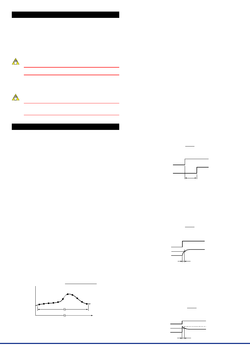
6.2 MXS-B Moving Average Computation
This computing unit stores the input values (X) sampled at intervals of
one-fortieth of the moving-average time (L) into 40 buffers in order,
and outputs the moving average of 40 input values (output-1 = Y1,
output-2 = Y2). The output between samplings is smoothed out by in-
terpolation. Minimum sampling time is the set computation cycle.
Therefore, when the moving-average time is set shorter, the number
of samplings is less than 40. When using a first-order lag filter for in-
put (X), set the first-order lag time constant (T).
Set the moving-average time (L) at % value in H02: CONST. The
value of 0 to 100.0% corresponds to that of 0 to 1000 seconds. For
example, enter “6” in H02 to set 60 seconds.
● Setting range of moving-average time:
0 to 320000 seconds (about 3.7 days) with 4 significant digits;
minimum unit is 1 second (however, 0.1 second for a setting of 4
seconds or shorter).
0.0 to 32000% can be set in H02.
( e.g. 12345% unacceptable, 12340% acceptable)
● Setting accuracy of moving-average time : ( ± 5.0% of set value)
±
1 second
Set the first-order lag time constant (T) at % value in H01: CONST.
The value of 0 to 100% corresponds to that of 0 to 100 seconds.
● Setting range of first-order lag time constant:
1.0 to 799.0 seconds; minimum unit is 0.1 second.
However, when not using the first-order lag function, set 0 sec-
ond.
● Setting accuracy of first-order lag time constant :
(
±
5.0% of set value)
±
1 second
X 40
X 39
X 38
X 37
X 36
X
35
X 5 X 4
X
3
X
2
X 1
Moving average=
Computation time
Time
X 1 +X 2 + • • • • • X 40
40 (Note)
Note: For the moving-average times at 3, 2 and 1
second, the number of samplings is 30, 20 and
10, respectively (when the computation cycle
is 100 ms).
6.3 MXS-C Dead Time Computation
This computing unit stores the input values (X) sampled at intervals of
one-fortieth of the dead time (L) into 40 buffers in order and outputs
data (output-1 = Y1, output-2 = Y2) after the dead time has elapsed.
Minimum sampling time is the set computation cycle. Therefore,
when the dead time is set shorter, the number of samplings is less
than 40. The output between samplings is smoothed out by interpola-
tion.
However, for the dead times of 3, 2 and 1 second, the number of sam-
plings is 30, 20, and 10, respectively (when the computation cycle is
100ms). When using a first-order lag filter for input (X), set the first-or-
der lag time constant (T).
Set the dead time (L) at % value in H02: CONST. The value of 0 to
100.0% corresponds to that of 0 to 1000 seconds. For example, enter
“6” in H02 to set 60 seconds.
● Setting range of dead time:
0 to 320000 seconds (about 3.7 days) with 4 significant digits;
minimum unit is 1 second (however, 0.1 second for a setting of
4 seconds or shorter). 0.0 to 32000% can be set in H02.
( e.g. 12345% unacceptable, 12340% acceptable)
● Setting accuracy of dead time: (
±
5.0% of set value)
±
1 second.
Set the first-order lag time constant (T) at % value in H01: CONST.
The value of 0 to 100% corresponds to that of 0 to 100 seconds.
● Setting range of first-order lag time constant:
1.0 to 799.0 seconds; the value of 1.0 to 799.0% corresponds to
that of 1.0 to 799.0 seconds; minimum unit is 0.1 second.
However, when not using the first-order lag function, set 0 sec-
ond.
● Setting accuracy of first-order lag time constant :
(
±
5.0% of set value)
±
1 second
Y1=Y2= X
e -L[s]
1+T[s]
e.g. 0%
→
100% step input
Input
Output
L
6.4 MXS-D First-order Lag Computation
This computing unit provides a first-order lag computation on input (X)
with a time constant (T) and outputs the result (output-1 = Y1, output-
2 = Y2). Set the time constant (T) at % value in H01: CONST. The
value of 0 to 100% corresponds to that of 0 to 100 seconds.
● Setting range of first-order lag time constant:
1.0 to 799.0 seconds; minimum unit is 0.1 second.
● Setting accuracy of first-order lag time constant :
(
± 5.0% of set value) ± 1 second
Y1=Y2= X
1
1+T[s]
e.g. 0% → 100% step input
Input 0%
63.2%
100%
100%
Output 0%
T
6.5 MXS-E First-order Lead Computation
This computing unit provides a first-order lead computation on input
(X) with a time constant (T) and outputs the result (output-1 = Y1, out-
put-2 = Y2). Set the time constant (T) at % value in H01: CONST. The
value of 0 to 100% corresponds to that of 0 to 100 seconds.
● Setting range of first-order lead time constant:
1.0 to 799.0 seconds; minimum unit is 0.1 second.
● Setting accuracy of first-order lead time constant :
(
±
5.0% of set value)
±
1 second
Y1=Y2= (1+ ) X
T[s]
1+T[s]
e.g. 0%
→
50% step input
Input 0%
68.4%
50%
100%
50%
Output 0%
T