Vernier Centripetal Force Apparatus - Manual (Page 6)

11
Data-Collection Overview and Software Setup
Sensors used with the CFA provide a reading of the force required to keep the
Sliding Carriage in position (the centripetal force) and the angular speed of the
rotating beam. Data can be collected from both sensors simultaneously, but the
software data-collection mode choices will depend on your goals and the particular
sensors chosen.
In order to discuss common data-collection modes used with this apparatus, let us
first examine a few experiments for context.
Experiments fall into two broad classes: exploration of centripetal force relations
(F=mv 2 /r, where v is the tangential velocity, or F=mr  2 , where ω is the angular
velocity) and moment of inertia experiments. We will concentrate here on centripetal
force.
Although the v 2 /r relationship is commonly encountered first in a physics
curriculum, the basic sensor measurement is angular speed. As a result, any software
configuration that reports tangential velocity will be more complex to implement,
because the student must provide the additional radius information in order for the
software to calculate tangential velocity from angular velocity (v= r). We
recommend the use of angular velocity for analysis with this apparatus.
Another data-collection subtlety is the behavior of photogate-based data collection
compared to time-based data collection. Most often with sensors, data collection is
time-based, where the sensor value is recorded at uniform time intervals, such as
every 0.02 seconds, or 50 times per second. Photogate data collection, in contrast, is
a record of times at which the gate state changes. These times will not be at regular
time intervals.
If force data are taken whenever the photogate records a transition (known as
Digital Events mode in Logger Pro), data will not be uniformly spaced. For most
analyses, unevenly spaced points will not matter. If force data are collected at
uniform time intervals, either the force or velocity data will have to be interpolated
in order to create a graph of force vs. velocity or velocity 2 .
Different combinations of sensors and interfaces will determine how data are best
collected. The Photogate always yields event times, even if other data collection is in
time-based mode. The WDSS and the Dual-Range Force Sensor can be used in
either time- or event-based data collection on LabQuest, but on Logger Pro the
WDSS must be used in time-based data collection.
The following sections give setup suggestions for a single experiment, centripetal
force vs. velocity (or velocity 2 ), using various sensor combinations, interfaces, and
either the angular velocity or the much simpler tangential velocity approach. We
suggest that you begin with one of our Logger Pro experiment files available in the
Probes and Sensors folder in Logger Pro version 3.8.5.1 and later.
12
Angular Velocity – Logger Pro 3 with Dual-Range Force Sensor
and Vernier Photogate
Open the file
CFA-DFS-Photogate-angular.cmbl.
This file is set up for a Dual-Range
Force Sensor and a Vernier Photogate.
The file contains the setup and a few
calculated columns that allow for easy
data collection. The data-collection
mode is time-based, which means that
the force readings will be taken at a
50 Hz rate, and the photogate readings
will happen as the Encoder Wheel
rotates. As a result, the force readings
are blank when there is a velocity
reading, and vice versa. This prevents
direct graphing of these columns, until
a simple calculation is done to provide
interpolated force values between the
regularly-spaced values.
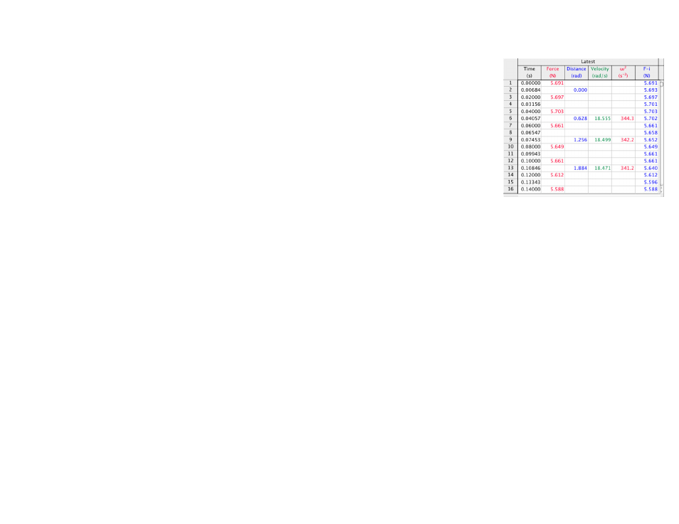
The column labeled “Force” contains the raw sensor values. The calculated column
“Force Interpolated,” or “F-i” for short, fills in the missing values. To see how we
defined the column, hover your mouse over the F-i column header in the data table
to see the definition. Any graphs between force and velocity must use the
F-i column.
The photogate is used to collect motion data of the object, where the “Distance”
column increments by a fixed amount for each block-to-block pair sensed by the
gate. Since the Encoder Wheel has ten slots, the increment is set to 0.628, with units
of radians, or 2π/10. The velocity (ω) column then has units of radians/second.
The file also contains a calculated column called “angular velocity 2 ,” or ω 2 for short.
This column is helpful in the data analysis, since a graph of F vs. ω 2 is a direct
proportionality of slope mr, given that F=mr  2 .
Connect an interface, Vernier Photogate, and Dual-Range Force Sensor, and reopen
the file CFA-DFS-Photogate-angular.cmbl. Place equal masses on the Sliding
Carriage and Counterbalance Carriage. Adjust the location of the force sensor so that
the Sliding Carriage will move in a circle of about a 10 cm radius, and set the
Counterbalance Carriage to a similar radius.
The current force reading is shown in the Logger Pro live readout. Spin the beam so
that the force reaches a reading of more than 5 N. This is most easily done by
spinning the shaft between the thumb and fingers. Start data collection.
Observe the Force-Interpolated vs. Time graph, and then display Force-Interpolated
vs. Angular Velocity. Also create and analyze a graph of Force-Interpolated vs.
Angular Velocity 2 .