3B Scientific 3B NETlab™ - Manual (Page 8)

8
generator can be set in the corresponding input
box of the “Sampling” panel. Next to this is the
check box “Generator enabled” that enables the
function generator.
The type of signal can be defined separately for
Channel A and Channel B by selecting the corre-
sponding output. Clicking “Predefined” opens a
dialog box in which one of the following prede-
fined signal waveforms can be selected: “Sine”,
“Rectangle”, “Triangle” and “Flat”. The parameters
are also modified according to the selected type of
signal. Click “OK” to confirm the entries. The speci-
fied signal is then displayed in a graphic.
It is possible to use the mouse to plot arbitrary
signal types on the graph. Move the cursor to the
left edge, press the left mouse button, draw the
desired signal with the cursor and release the
mouse button after you have finished.
The period and frequency of a repeating signal are
displayed above the graphic.
If the same signal is to be output to both outputs,
set the signal for output A and click “Copy from A”
under “Channel B” (or vice versa).
Note that the function generator is not working in
the oscilloscope mode.
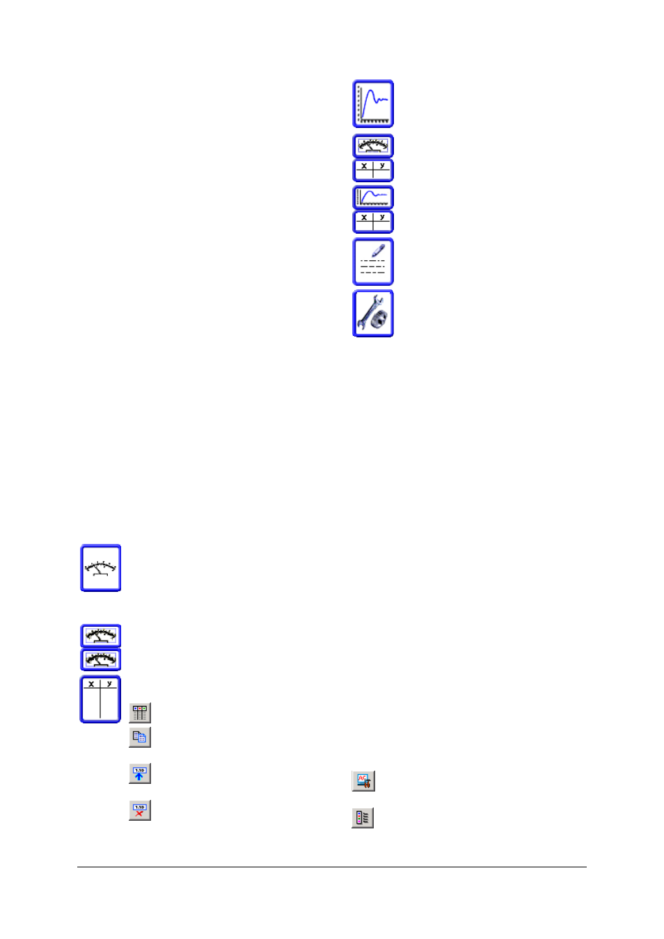
5.1.8 Evaluation:
5.1.8.1 Display of measurements:
After any measurement in standard or oscilloscope
mode, the data can be viewed in various forms. It is
possible to change the display at any given time by
simply clicking the corresponding icons at the top
edge of the screen.
Dial: the current value is displayed on a
dial as on an analog multimeter. This
representation is useful at slow speeds or
in manual mode because the currently
valid measurement can be displayed in
real time.
Dual display: the values of two inputs
are displayed simultaneously.
Table: a table containing the measured
values is displayed
Selects the columns to be displayed
Copies the selected measured data
records to the clipboard
Manual entry of values in the se-
lected cells
Deletes all manually entered values
Graph: the measured values are plotted
on a graph. The next section deals with
the functions available for the graphical
display.
Table and pointer: see above
Graph and table: see above
Notes: This allows you to enter com-
ments describing the measurements.
Settings: once a display setting for the
left-hand side of the screen has been
configured, clicking this icon allows the
control fields to be reopened for modifi-
cation.
5.1.8.2 Graphical display:
In a graphical display, the data for each digital
input is displayed in a different colour with a leg-
end underneath. The parameters for the x-axis are
entered in the first row.
The graph provides two cursors represented by
vertical dotted lines that can be moved along the x-
axis. Just move the mouse close to one of these
cursors, press the left mouse button and move the
cursor to the requisite position, releasing the cursor
when it is correctly placed. The coordinates of the
cursor are displayed in the row containing the
legend for the x-axis. Beneath that, the individual
measurements are contained in the rows corre-
sponding to the y-axis, i.e. the y coordinates for the
selected curve at the cursor position.
The right mouse button is used for zooming. A
context menu appears which provide the possibility
of zooming in or out of the x-axis, the y-axis or
both of the axes. It is possible to highlight sections
by keeping the right mouse button pressed and
dragging the mouse, thereby enclosing the relevant
section in a rectangle. The contents highlighted
within this rectangle can be magnified to fill the
entire screen by selecting “Zoom into selected win-
dow”. The visible section of the graph can be
shifted by dragging the axis legend with the left
mouse button.
A row of icons is located above the graph. The
following sections explain their function:
Setup display: (connecting lines, grids, data
points, etc.)
Select inputs/formulas to be displayed: also
for assigning what is to be on the x-axis. The x-axis